| POV-Ray for Unix version 3.7 | ||||
|
|
||||
| Home | POV-Ray for Unix | POV-Ray Tutorial | POV-Ray Reference | |
3.4 Scene File Elements
This section details settings, camera types, objects, and textures used in POV-Ray scene files. It is divided into the following sub-sections:
3.4.1 Global Settings
The global_settings statement is a catch-all statement that
gathers together a number of global parameters. The statement may appear
anywhere in a scene as long as it is not inside any other statement. You may
have multiple global_settings statements in a scene. Whatever
values were specified in the last global_settings statement
override any previous settings.
Note: Some items which were language directives in earlier versions of
POV-Ray have been moved inside the global_settings statement so
that it is more obvious to the user that their effect is global. The old
syntax is permitted but generates a warning.
The new syntax is:
GLOBAL_SETTINGS:
  global_settings { [GLOBAL_SETTINGS_ITEMS...] }
GLOBAL_SETTINGS_ITEM:
  adc_bailout Value | ambient_light COLOR | assumed_gamma GAMMA_VALUE |
  hf_gray_16 [Bool] | irid_wavelength COLOR | charset GLOBAL_CHARSET |
  max_intersections Number | max_trace_level Number |
  mm_per_unit Number | number_of_waves Number | noise_generator Number |
  radiosity { RADIOSITY_ITEMS... } | subsurface { SUBSURFACE_ITEMS } |
  photon { PHOTON_ITEMS... }
GLOBAL_CHARSET:
  ascii | utf8 | sys
GAMMA_VALUE:
  Value | srgb
Global setting default values:
charset		   : ascii
adc_bailout	   : 1/255
ambient_light	   : <1,1,1>
assumed_gamma	   : 1.0 (undefined for legacy scenes)
hf_gray_16	   : deprecated
irid_wavelength	   : <0.25,0.18,0.14>
max_trace_level	   : 5
max_intersections  : 64
mm_per_unit        : 10
number_of_waves	   : 10
noise_generator	   : 2

Radiosity:
adc_bailout	   : 0.01
always_sample	   : off
brightness	   : 1.0
count		   : 35  (supports adaptive mode)
error_bound	   : 1.8
gray_threshold	   : 0.0
low_error_factor   : 0.5
max_sample	   : non-positive value
maximum_reuse      : 0.2
minimum_reuse	   : 0.015
nearest_count	   : 5   (max = 20; supports adaptive mode)
normal		   : off
pretrace_start	   : 0.08
pretrace_end	   : 0.04
recursion_limit	   : 2
subsurface 	   : off

Subsurface:
radiosity	   : off
samples		   : 50,50
Each item is optional and may appear in any order. If an item is specified more than once, the last setting overrides previous values. Details on each item are given in the following sections.
3.4.1.1 ADC_Bailout
In scenes with many reflective and transparent surfaces, POV-Ray can get bogged down tracing multiple reflections and refractions that contribute very little to the color of a particular pixel. The program uses a system called Adaptive Depth Control (ADC) to stop computing additional reflected or refracted rays when their contribution is insignificant.
You may use the global setting adc_bailout keyword followed by
float value to specify the point at which a ray's contribution is
considered insignificant. For example:
global_settings { adc_bailout 0.01 }
The default value is 1/255, or approximately 0.0039, since a change
smaller than that could not be visible in a 24 bit image. Generally this
setting is perfectly adequate and should be left alone. Setting
adc_bailout to 0 will disable ADC, relying completely on
max_trace_level to set an upper limit on the number of rays spawned.
See the section Max_Trace_Level for details on how ADC and max_trace_level interact.
3.4.1.2 Ambient_Light
Ambient light is used to simulate the effect of inter-diffuse reflection
that is responsible for lighting areas that partially or completely lie in
shadow. POV-Ray provides the ambient_light keyword to let you
easily change the brightness of the ambient lighting without changing every
ambient value in all finish statements. It also lets you create interesting
effects by changing the color of the ambient light source. The syntax is:
global_settings { ambient_light COLOR }
The default is a white ambient light source set at rgb
<1,1,1>. Only the rgb components are used. The actual ambient
used is: Ambient = Finish_Ambient * Global_Ambient.
See the section Ambient for more information.
3.4.1.3 Assumed_Gamma
The assumed_gamma statement specifies a dsiplay gamma for which all color literals in the scene are presumed to be pre-corrected; at the same time it also defines the working gamma space in which POV-Ray will perform all its color computations.
Note: Using any value other than 1.0 will produce physically inaccurate results. Furthermore, if you decide to go for a different value for convenience, it is highly recommended to set this value to the same as your Display_Gamma. Using this parameter for artistic purposes is strongly discouraged.
Note: As of POV-Ray 3.7 this keyword is considered mandatory (except in legacy scenes) and consequently enables the experimental gamma handling feature. Future versions of POV-Ray may treat the absence of this keyword in non-legacy scenes as an error.
See section Gamma Handling for more information about gamma.
3.4.1.4 HF_Gray_16
Grayscale output can be used to generate heightfields for use in other POV-Ray scenes, and may be specified via Grayscale_Output=true as an INI option, or +Fxg (for output type 'x') as a command-line option. For example, +Fng for PNG and +Fpg for PPM (effectively PGM) grayscale output. By default this option is off.
Note: In version 3.7 the hf_gray_16 keyword in the global_settings block has been deprecated. If encountered, it has no effect on the output type and will additionally generate a warning message.
With Grayscale_Output=true, the output file will be in the form of a heightfield, with the height at any point being dependent on the brightness of the pixel. The brightness of a pixel is calculated in the same way that color images are converted to grayscale images: height = 0.3 * red + 0.59 * green + 0.11 * blue.
Setting the Grayscale_Output=true option will cause the preview display, if used, to be grayscale rather than color. This is to allow you to see how the heightfield will look because some file formats store heightfields in a way that is difficult to understand afterwards. See the section Height Field for a description of how POV-Ray heightfields are stored for each file type.
Caveat: Grayscale output implies the maximum bit-depth the format supports is 16, it is not valid to specify bits per color channel with 'g' (e.g. +Fng16 is not allowed, and nor for that matter is +Fn16g). If bits per channel is provided via an INI option, it is ignored.
Currently PNG, and PPM are the only file formats that support grayscale output.
3.4.1.5 Irid_Wavelength
Iridescence calculations depend upon the dominant wavelengths of the
primary colors of red, green and blue light. You may adjust the values using
the global setting irid_wavelength as follows...
global_settings { irid_wavelength COLOR }
The default value is rgb <0.70,0.52,0.48> and any
filter or transmit values are ignored. These values are proportional to the
wavelength of light but they represent no real world units.
In general, the default values should prove adequate but we provide this option as a means to experiment with other values.
3.4.1.6 Charset
This allows you to specify the assumed character set of all text strings.
If you specify ascii only standard ASCII character codes in the
range from 0 to 127 are valid. You can easily find a table of ASCII
characters on the internet. The option utf8 is a special Unicode
text encoding and it allows you to specify characters of nearly all languages
in use today. We suggest you use a text editor with the capability to export
text to UTF8 to generate input files. You can find more information,
including tables with codes of valid characters on the
Unicode website
The last possible option is to use a system specific character set. For
details about the sys character set option refer to the platform
specific documentation.
3.4.1.7 Max_Trace_Level
In scenes with many reflective and transparent surfaces POV-Ray can get
bogged down tracing multiple reflections and refractions that contribute very
little to the color of a particular pixel. The global setting
max_trace_level defines the integer maximum number of recursive levels
that POV-Ray will trace a ray.
global_settings { max_trace_level Level }
This is used when a ray is reflected or is passing through a transparent object and when shadow rays are cast. When a ray hits a reflective surface, it spawns another ray to see what that point reflects. That is trace level one. If it hits another reflective surface another ray is spawned and it goes to trace level two. The maximum level by default is five.
One speed enhancement added to POV-Ray in version 3.0 is Adaptive Depth
Control (ADC). Each time a new ray is spawned as a result of reflection
or refraction its contribution to the overall color of the pixel is reduced
by the amount of reflection or the filter value of the refractive surface. At
some point this contribution can be considered to be insignificant and there
is no point in tracing any more rays. Adaptive depth control is what tracks
this contribution and makes the decision of when to bail out. On scenes that
use a lot of partially reflective or refractive surfaces this can result in a
considerable reduction in the number of rays fired and makes it safer to use
much higher max_trace_level values.
This reduction in color contribution is a result of scaling by the
reflection amount and/or the filter values of each surface, so a perfect
mirror or perfectly clear surface will not be optimizable by ADC. You can see
the results of ADC by watching the Rays Saved and Highest
Trace Level displays on the statistics screen.
The point at which a ray's contribution is considered insignificant is
controlled by the adc_bailout value. The default is 1/255 or
approximately 0.0039 since a change smaller than that could not be visible in
a 24 bit image. Generally this setting is perfectly adequate and should be
left alone. Setting adc_bailout to 0 will disable ADC, relying
completely on max_trace_level to set an upper limit on the
number of rays spawned.
If max_trace_level is reached before a non-reflecting surface
is found and if ADC has not allowed an early exit from the ray tree the
color is returned as black. Raise max_trace_level if you see
black areas in a reflective surface where there should be a color.
The other symptom you could see is with transparent objects. For instance,
try making a union of concentric spheres with a clear texture on them. Make
ten of them in the union with radius's from 1 to 10 and render the scene.
The image will show the first few spheres correctly, then black. This is
because a new level is used every time you pass through a transparent
surface. Raise max_trace_level to fix this problem.
Note: Raising max_trace_level will use more memory and time
and it could cause the program to crash with a stack overflow error, although
ADC will alleviate this to a large extent.
Values for max_trace_level can be set up to a maximum of 256.
If there is no max_trace_level set and during rendering the default value is reached, a warning is issued.
3.4.1.8 Max_Intersections
POV-Ray uses a set of internal stacks to collect ray/object intersection points. The usual maximum number of entries in these I-Stacks is 64. Complex scenes may cause these stacks to overflow. POV-Ray does not stop but it may incorrectly render your scene. When POV-Ray finishes rendering, a number of statistics are displayed. If you see I-Stack overflows reported in the statistics you should increase the stack size. Add a global setting to your scene as follows:
global_settings { max_intersections Integer }
If the I-Stack Overflows remain increase this value until they stop.
3.4.1.9 Mm_Per_Unit
See the section Subsurface Light Transport for more information about the role of mm_per_unit in the global settings block.
3.4.1.10 Number_Of_Waves
The waves and ripples
patterns are generated by summing a series of waves, each with a slightly different center and size. By default, ten waves are summed but this amount can be globally controlled by changing the number_of_waves setting.
global_settings { number_of_waves Integer }
Changing this value affects both waves and ripples alike on all patterns in the scene.
3.4.1.11 Noise_generator
There are three noise generators implemented.
noise_generator 1the noise that was used in POV_Ray 3.1noise_generator 2'range corrected' version of the old noise, it does not show the plateaus seen withnoise_generator 1noise_generator 3generates Perlin noise
The default is noise_generator 2
Note: The noise_generators can also be used within the pigment/normal/etc. statement.
3.4.1.12 Subsurface
See the section Subsurface Light Transport for more information about the role of subsurface in the global settings block.
3.4.2 Camera
The camera definition describes the position, projection type and properties of the camera viewing the scene. Its syntax is:
CAMERA:
  camera{ [CAMERA_ITEMS...] }
CAMERA_ITEMS:
  CAMERA_TYPE | CAMERA_VECTOR | CAMERA_MODIFIER |
  CAMERA_IDENTIFIER
CAMERA_TYPE:
  perspective | orthographic | mesh_camera{MESHCAM_MODIFIERS} | fisheye | ultra_wide_angle |
  omnimax | panoramic | cylinder CylinderType | spherical
CAMERA_VECTOR:
  location <Location> | right <Right> | up <Up> |
  direction <Direction> | sky <Sky>
CAMERA_MODIFIER:
  angle HORIZONTAL [VERTICAL] | look_at <Look_At> |
  blur_samples [MIN_SAMPLES,] MAX_SAMPLES | aperture Size |
  focal_point <Point> | confidence Blur_Confidence |
  variance Blur_Variance | [bokeh{pigment{BOKEH}}] |
  NORMAL | TRANSFORMATION | [MESHCAM_SMOOTH]
MESHCAM_MODIFIERS:
  rays per pixel & distribution type & [max distance] & MESH_OBJECT & [MESH_OBJECT...]
BOKEH:
  a COLOR_VECTOR in the range of <0,0,0> ... <1,1,0>
MESHCAM_SMOOTH:
  optional smooth modifier valid only when using mesh_camera
Camera default values:
DEFAULT CAMERA:
camera {
  perspective
  location <0,0,0>
  direction <0,0,1>
  right 1.33*x
  up y
  sky <0,1,0>
  }

CAMERA TYPE: perspective
  angle      : ~67.380 ( direction_length=0.5*
             right_length/tan(angle/2) )
  confidence : 0.9 (90%)
  direction  : <0,0,1>
  focal_point: <0,0,0>
  location   : <0,0,0>
  look_at    : z
  right      : 1.33*x
  sky        : <0,1,0>
  up         : y
  variance   : 1/128
Depending on the projection type zero or more of the parameters are required:
- If no camera is specified the default camera is used.
- If no projection type is given the perspective camera will be used (pinhole camera).
- The CAMERA_TYPE has to be the first item in the camera statement.
- Other CAMERA_ITEMs may legally appear in any order.
- For other than the perspective camera, the minimum that has to be specified is the CAMERA_TYPE, the cylindrical camera also requires the CAMERA_TYPE to be followed by a float.
- The Orthographic camera has two 'modes'. For the pure orthographic projection up or right have to be specified. For an orthographic camera, with the same area of view as a perspective camera at the plane which goes through the look_at point, the angle keyword has to be use. A value for the angle is optional.
- All other CAMERA_ITEMs are taken from the default camera, unless they are specified differently.
3.4.2.1 Placing the Camera
The POV-Ray camera has 9 different models and they are as follows:
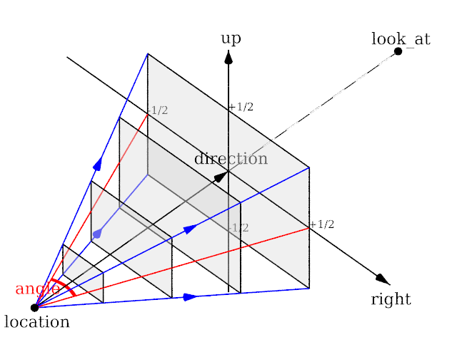
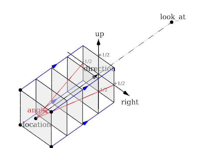
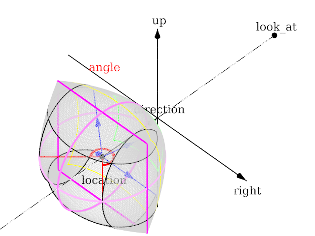
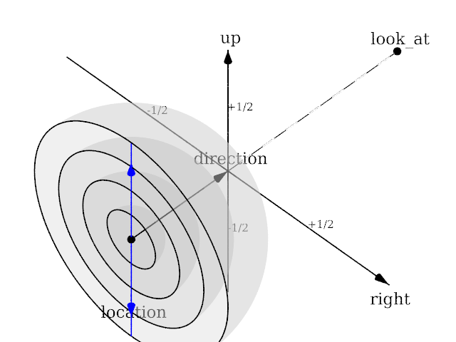
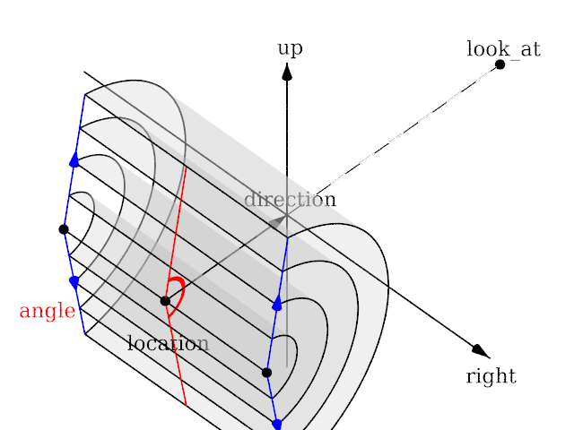
Each of which uses a different projection method to project the scene onto your screen. Regardless of the projection type all cameras use location, right, up, direction, and other keywords to determine the location and orientation of the camera. The type keywords and these four vectors fully define the camera. All other camera modifiers adjust how the camera does its job. The meaning of these vectors and other modifiers differ with the projection type used. A more detailed explanation of the camera types follows later. In the sub-sections which follows, we explain how to place and orient the camera by the use of these four vectors and the sky and look_at modifiers. You may wish to refer to the illustration of the perspective camera below as you read about these
vectors.
|
|
Basic (default) camera geometry |
3.4.2.1.1 Location and Look_At
Under many circumstances just two vectors in the camera statement are all
you need to position the camera: location and look_at
vectors. For example:
camera {
  location <3,5,-10>
  look_at <0,2,1>
  }
The location is simply the x, y, z coordinates of the camera. The camera
can be located anywhere in the ray-tracing universe. The default location is
<0,0,0>. The look_at vector tells POV-Ray to
pan and tilt the camera until it is looking at the specified x, y, z
coordinates. By default the camera looks at a point one unit in the
z-direction from the location.
The look_at modifier should almost always be the last item in
the camera statement. If other camera items are placed after the
look_at vector then the camera may not continue to look at the
specified point.
3.4.2.1.2 The Sky Vector
Normally POV-Ray pans left or right by rotating about the y-axis until it
lines up with the look_at point and then tilts straight up or
down until the point is met exactly. However you may want to slant the camera
sideways like an airplane making a banked turn. You may change the tilt of
the camera using the sky vector. For example:
camera {
  location <3,5,-10>
  sky   <1,1,0>
  look_at <0,2,1>
  }
This tells POV-Ray to roll the camera until the top of the camera is in
line with the sky vector. Imagine that the sky vector is an antenna pointing
out of the top of the camera. Then it uses the sky vector as the
axis of rotation left or right and then to tilt up or down in line with the
sky until pointing at the look_at point. In effect
you are telling POV-Ray to assume that the sky isn't straight up.
The sky vector does nothing on its own. It only modifies the
way the look_at vector turns the camera. The default value is
sky<0,1,0>.
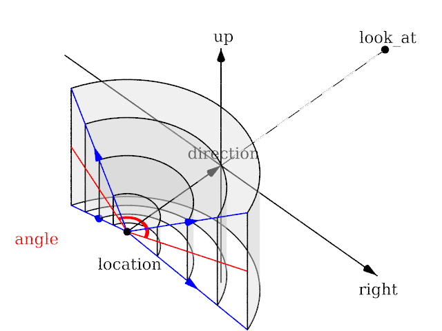
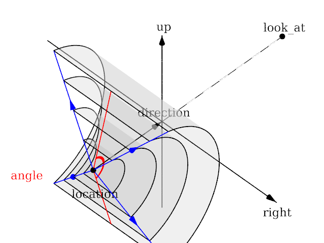
3.4.2.1.3 Angles
The angle keyword followed by a float expression specifies
the (horizontal) viewing angle in degrees of the camera used. Even though it
is possible to use the direction vector to determine the viewing
angle for the perspective camera it is much easier to use the
angle keyword.
When you specify the angle, POV-Ray adjusts the length of the
direction vector accordingly. The formula used is
direction_length = 0.5 * right_length / tan(angle / 2) where
right_length is the length of the right vector. You should
therefore specify the direction and right vectors
before the angle keyword. The right vector is
explained in the next section.
There is no limitation to the viewing angle except for the perspective projection. If you choose viewing angles larger than 360 degrees you will see repeated images of the scene (the way the repetition takes place depends on the camera). This might be useful for special effects.
The spherical camera has the option to also specify a vertical
angle. If not specified it defaults to the horizontal angle/2
For example if you render an image with a 2:1 aspect ratio and map it to a sphere using spherical mapping, it will recreate the scene. Another use is to map it onto an object and if you specify transformations for the object before the texture, say in an animation, it will look like reflections of the environment (sometimes called environment mapping).
3.4.2.1.4 The Direction Vector
You will probably not need to explicitly specify or change the camera
direction vector but it is described here in case you do. It
tells POV-Ray the initial direction to point the camera before moving it with
the look_at or rotate vectors (the default value is
direction<0,0,1>). It may also be used to control the
(horizontal) field of view with some types of projection. The length of the
vector determines the distance of the viewing plane from the camera's
location. A shorter direction vector gives a wider view while a
longer vector zooms in for close-ups. In early versions of POV-Ray, this was
the only way to adjust field of view. However zooming should now be done
using the easier to use angle keyword.
If you are using the ultra_wide_angle, panoramic,
or cylindrical projection you should use a unit length
direction vector to avoid strange results. The length of the
direction vector does not matter when using the
orthographic, fisheye, or omnimax projection
types.
3.4.2.1.5 Up and Right Vectors
The primary purpose of the up and right vectors
is to tell POV-Ray the relative height and width of the view screen. The
default values are:
right 4/3*x
up y
In the default perspective camera, these two vectors also
define the initial plane of the view screen before moving it with the
look_at or rotate vectors. The length of the
right vector (together with the direction vector) may
also be used to control the (horizontal) field of view with some types of
projection. The look_at modifier changes both the up
and right vectors. The angle calculation depends on the
right vector.
Most camera types treat the up and right vectors
the same as the perspective type. However several make special
use of them. In the orthographic projection: The lengths of the
up and right vectors set the size of the viewing
window regardless of the direction vector length, which is not
used by the orthographic camera.
When using cylindrical projection: types 1 and 3, the axis of
the cylinder lies along the up vector and the width is
determined by the length of right vector or it may be overridden
with the angle vector. In type 3 the up vector
determines how many units high the image is. For example if you have up
4*y on a camera at the origin. Only points from y=2 to y=-2 are
visible. All viewing rays are perpendicular to the y-axis. For type 2 and 4,
the cylinder lies along the right vector. Viewing rays for type
4 are perpendicular to the right vector.
Note: The up, right, and direction vectors should always remain perpendicular to each other or the image will be distorted. If this is not the case a warning message will be printed. The vista buffer will not work for non-perpendicular camera vectors.
3.4.2.1.6 Aspect Ratio
Together the up and right vectors define the
aspect ratio (height to width ratio) of the resulting image. The
default values up<0,1,0> and
right<1.33,0,0> result in an aspect ratio of 4 to 3. This is the
aspect ratio of a typical computer monitor. If you wanted a tall skinny image
or a short wide panoramic image or a perfectly square image you should adjust
the up and right vectors to the appropriate
proportions.
Most computer video modes and graphics printers use perfectly square pixels.
For example Macintosh displays and IBM SVGA modes 640x480, 800x600 and
1024x768 all use square pixels. When your intended viewing method uses square
pixels then the width and height you set with the Width and
Height options or +W or +H switches
should also have the same ratio as the up and right
vectors.
Note: 640/480 = 4/3 so the ratio is proper for this square pixel mode.
Not all display modes use square pixels however. For example IBM VGA mode
320x200 and Amiga 320x400 modes do not use square pixels. These two modes
still produce a 4/3 aspect ratio image. Therefore images intended to be
viewed on such hardware should still use 4/3 ratio on their up
and right vectors but the pixel settings will not be 4/3.
For example:
camera {
  location <3,5,-10>
  up    <0,1,0>
  right  <1,0,0>
  look_at <0,2,1>
  }
This specifies a perfectly square image. On a square pixel display like
SVGA you would use pixel settings such as +W480 +H480 or
+W600 +H600. However on the non-square pixel Amiga 320x400 mode you
would want to use values of +W240 +H400 to render a square
image.
The bottom line issue is this: the up and right
vectors should specify the artist's intended aspect ratio for the image
and the pixel settings should be adjusted to that same ratio for square
pixels and to an adjusted pixel resolution for non-square pixels. The
up and right vectors should not be adjusted
based on non-square pixels.
3.4.2.1.7 Handedness
The right vector also describes the direction to the right of
the camera. It tells POV-Ray where the right side of your screen is. The sign
of the right vector can be used to determine the handedness of
the coordinate system in use. The default value is:
right<1.33,0,0>. This means that the +x-direction is to the
right. It is called a left-handed system because you can use your
left hand to keep track of the axes. Hold out your left hand with your palm
facing to your right. Stick your thumb up. Point straight ahead with your
index finger. Point your other fingers to the right. Your bent fingers are
pointing to the +x-direction. Your thumb now points into +y-direction. Your
index finger points into the +z-direction.
To use a right-handed coordinate system, as is popular in some CAD programs
and other ray-tracers, make the same shape using your right hand. Your thumb
still points up in the +y-direction and your index finger still points
forward in the +z-direction but your other fingers now say the +x-direction
is to the left. That means that the right side of your screen is now in the
-x-direction. To tell POV-Ray to act like this you can use a negative x value
in the right vector such as:
right<-1.33,0,0>. Since having x values increasing to the left
does not make much sense on a 2D screen you now rotate the whole thing 180
degrees around by using a positive z value in your camera's location. You
end up with something like this.
camera {
  location <0,0,10>
  up    <0,1,0>
  right  <-1.33,0,0>
  look_at <0,0,0>
  }
Now when you do your ray-tracer's aerobics, as explained in the section Understanding POV-Ray's Coordinate System, you use your right hand to determine the direction of rotations.
In a two dimensional grid, x is always to the right and y is up. The two versions of handedness arise from the question of whether z points into the screen or out of it and which axis in your computer model relates to up in the real world.
Architectural CAD systems, like AutoCAD, tend to use the God's Eye orientation that the z-axis is the elevation and is the model's up direction. This approach makes sense if you are an architect looking at a building blueprint on a computer screen. z means up, and it increases towards you, with x and y still across and up the screen. This is the basic right handed system.
Stand alone rendering systems, like POV-Ray, tend to consider you as a participant. You are looking at the screen as if you were a photographer standing in the scene. The up direction in the model is now y, the same as up in the real world and x is still to the right, so z must be depth, which increases away from you into the screen. This is the basic left handed system.
3.4.2.1.8 Transforming the Camera
The various transformations such as translate and
rotate modifiers can re-position the camera once you have defined
it. For example:
camera {
  location < 0, 0, 0>
  direction < 0, 0, 1>
  up    < 0, 1, 0>
  right   < 1, 0, 0>
  rotate  <30, 60, 30>
  translate < 5, 3, 4>
  }
In this example, the camera is created, then rotated by 30 degrees about the x-axis, 60 degrees about the y-axis and 30 degrees about the z-axis, then translated to another point in space.
3.4.2.2 Types of Projection
|
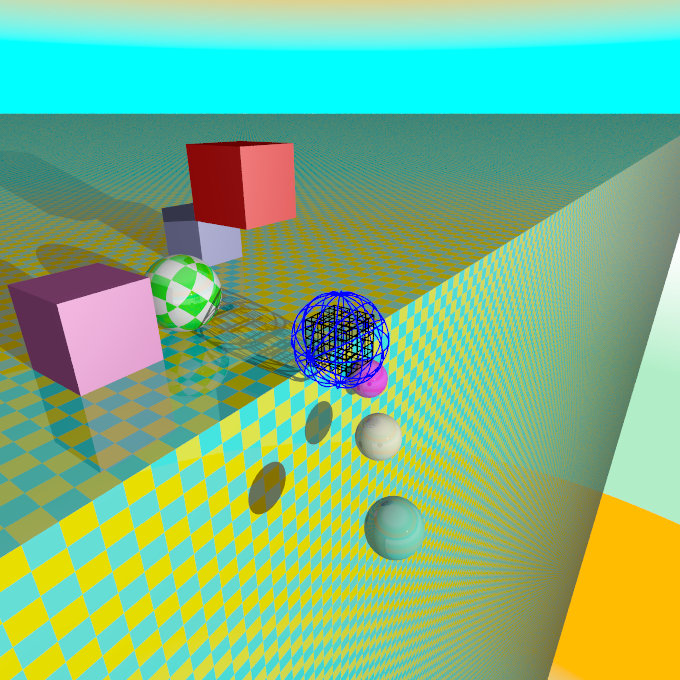
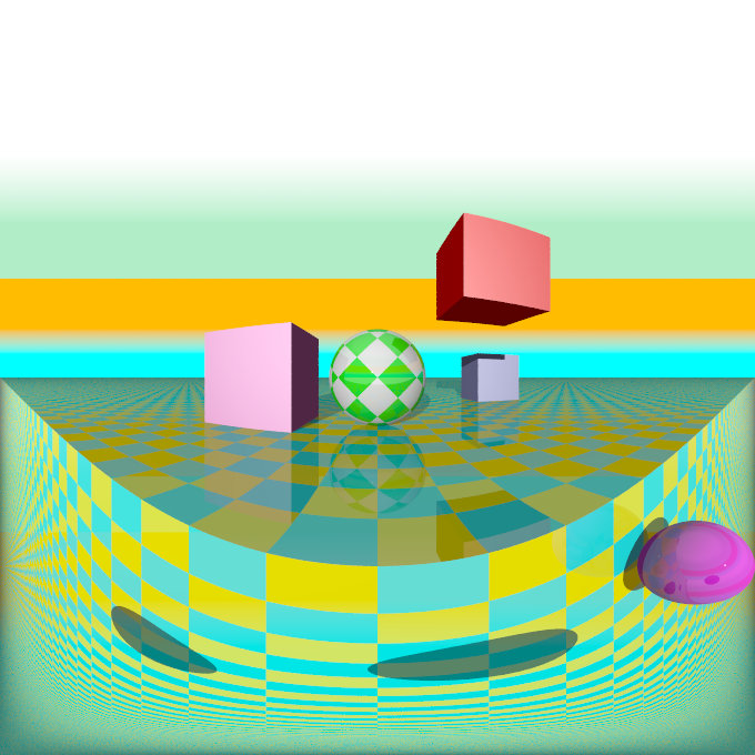
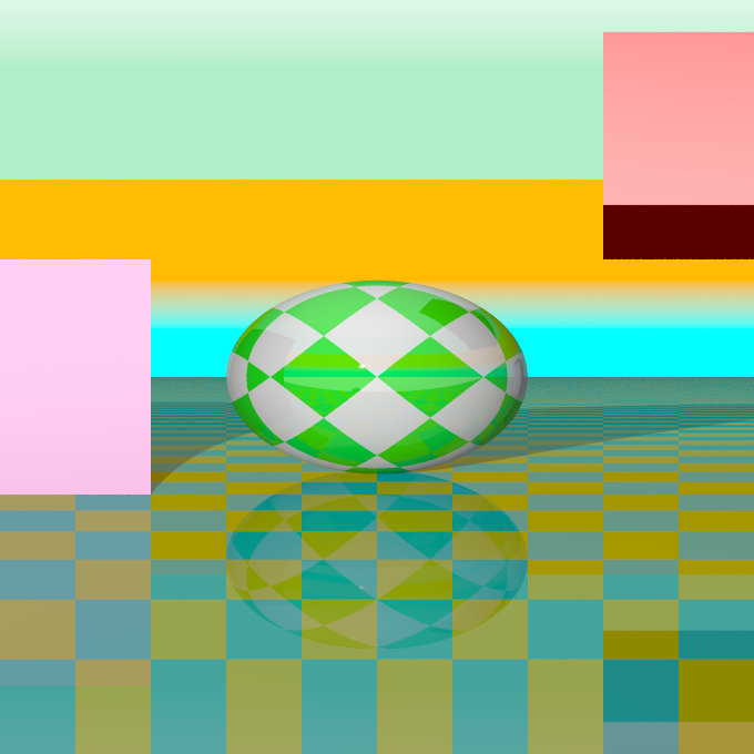
The following sections explain the different projection types that can be used with the scene camera. The most common types are the perspective and orthographic projections. The CAMERA_TYPE should be the first item in a |
|
The camera sample scene global view |
Note: The vista buffer feature can only be used with the perspective and orthographic camera.
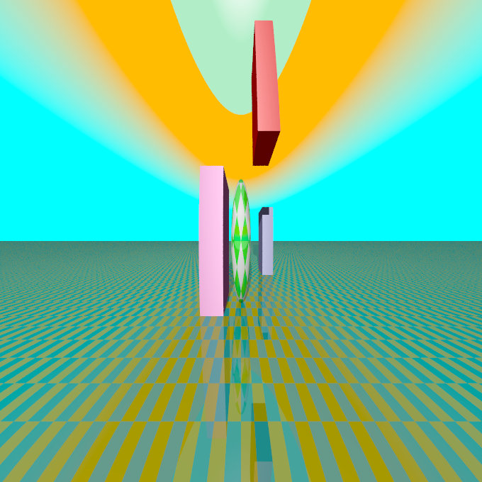
3.4.2.2.1 Perspective projection
The perspective keyword specifies the default perspective camera which simulates the classic pinhole camera. The horizontal viewing angle is either determined by the ratio between the length of the direction vector and the length of the right vector or by the optional keyword angle, which is the preferred way. The viewing angle has to be larger than 0 degrees and smaller than 180 degrees.
|
|
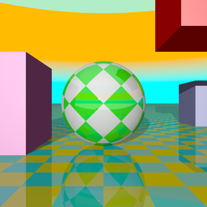
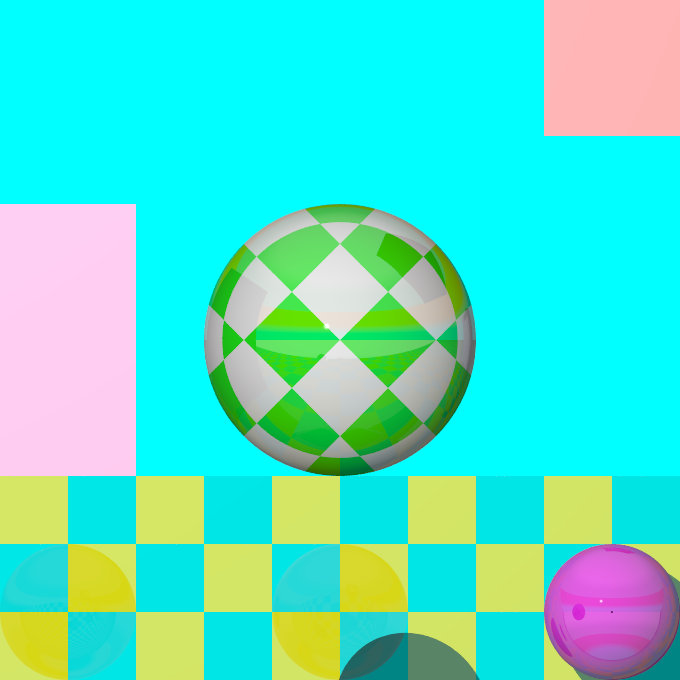
|
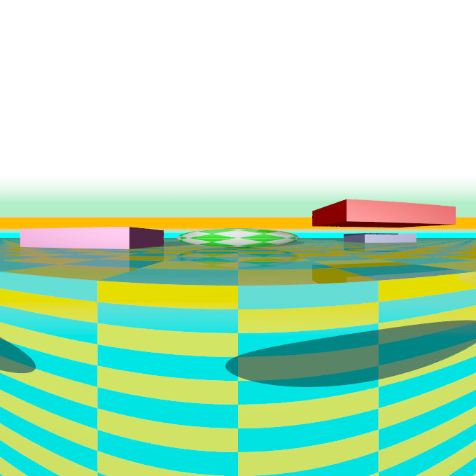
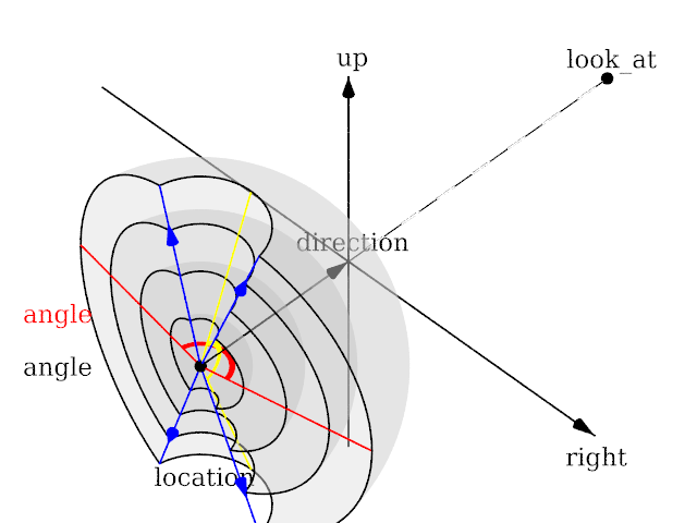
The perspective projection diagram |
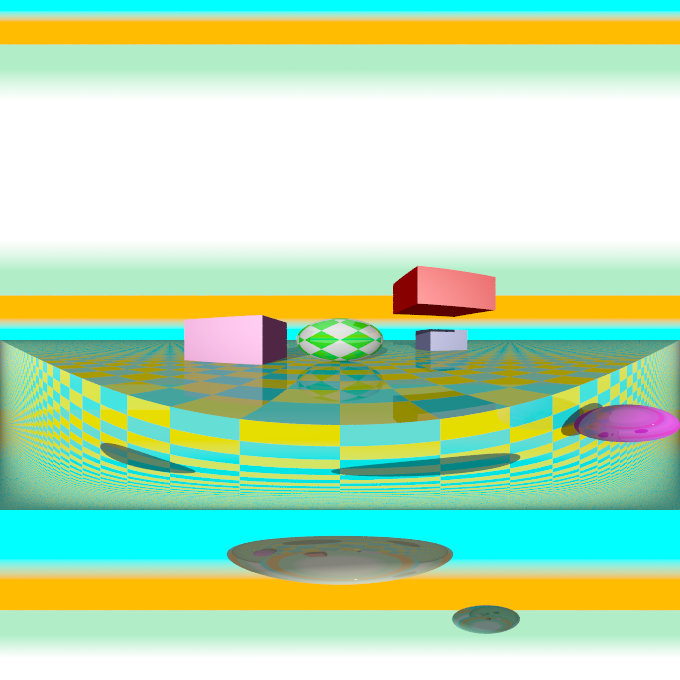
A perspective camera sample image |
Note: The angle keyword can be used as long as less than 180 degrees. It recomputes the length of right and up vectors using direction. The proper aspect ratio between the up and right vectors is maintained.
3.4.2.2.2 Orthographic projection
The orthographic camera offers two modes of operation:
The pure orthographic projection. This projection uses parallel camera rays to create an image of the scene. The area of view is determined by the lengths of the right and up vectors. One of these has to be specified, they are not taken from the default camera. If omitted the second method of the camera is used.
If, in a perspective camera, you replace the perspective keyword by orthographic and leave all other parameters the same, you will get an orthographic view with the same image area, i.e. the size of the image is
the same. The same can be achieved by adding the angle keyword to an orthographic camera. A value for the angle is optional. So this second mode is active if no up and right are within the camera statement, or when the angle keyword is within the camera statement.
You should be aware though that the visible parts of the scene change when switching from perspective to orthographic view. As long as all objects of interest are near the look_at point they will be still visible if the orthographic camera is used. Objects farther away may get out of view while nearer objects will stay in view.
If objects are too close to the camera location they may disappear. Too close here means, behind the orthographic camera projection plane (the plane that goes through the location point).
|
|
|
The orthographic projection diagram |
An orthographic camera sample image |
Note: The length of direction is irrelevant unless angle is used. The lengths of up and right define the dimensions of the view. The angle keyword can be used, as long as less than 180. It will override the length of the right and up vectors (the aspect ratio between up and right will be kept nevertheless) with a scope of a perspective camera having the same direction and angle.
3.4.2.2.3 Mesh projection
The mesh projection is a special camera type that allows complete control of the ray origin and direction for each pixel of the output image. The basic concept is to associate pixels with faces defined within a previously declared mesh or mesh2 object. The MESH_OBJECT_IDENTIFIER need not be instantiated in the scene, though it can be, and doing so can lead to some interesting uses, such as texture baking or illumination calculations.
In its simplest form, each pixel of the output image is assigned to a face of the mesh according to (width * (int) y) + (int) x, however, more complex mapping is possible via multiple meshes and multiple rays per pixel. The type of mapping in use is determined by the distribution type parameter in the camera declaration. Except for mapping #3, the ray origin will be set to the centroid of the face, and the direction will be that of the face's normal. For mapping #3, barycentric co-ordinates are determined from the UV co-ordinates of the first face to match the X and Y position, and those are then converted to a position on the face which will serve as the ray origin. Support is provided to move the origin off the face along the normal, and to reverse the ray direction.
For most of the distribution methods, any POV feature that causes sub-pixel positioning to be used for shooting rays (e.g. anti-aliasing or jitter) will not do anything useful, because X and Y are converted to integers for indexing purposes. At this time, no warning is issued if anti-aliasing or jitter is requested when rendering a non-applicable distribution; this may be added later.
The syntax for the mesh camera is as follows:
camera {
  mesh_camera {
    rays per pixel
    distribution type
    [max distance]
    mesh {
      MESH_OBJECT_IDENTIFIER
      [TRANSFORMATIONS]
    }
    [mesh ...]
  }
  [location]
  [direction]
  [smooth]
  }
Note: The mesh camera is an experimental feature introduced in version 3.7 beta 39 and its syntax is likely to change. Additionally, many of the normal camera concepts presented in this section (such as location and direction) either do not work as they do for other cameras or do not work at all (for example, the concept of 'up' simply does not apply to a mesh camera). It should also be kept in mind that the camera has not yet been tested with many of POV-Ray's advanced features such as photons and radiosity, and more work in that area is likely to be needed.
3.4.2.2.3.1 Rays Per Pixel
This float parameter controls the number of rays that will be shot for each pixel in the output image. Each distribution allows different values, but the minimum is always 1.
3.4.2.2.3.2 Distribution Type
This float parameter controls how pixels are assigned to faces as documented below:
- distribution #0
This method allows single or multiple rays per pixel, with the ray number for that pixel allocated to each mesh in turn. The index into the meshes is the ray number, where rays per pixel is greater than one, and the index into the selected mesh is the pixel number within the output image. If there is no face at that pixel position, the resulting output pixel is unaffected.
You must supply at least as many meshes as rays per pixel. Each pixel is shot rays per pixel times, and the results averaged. Any ray that does not correspond with a face (i.e. the pixel number is greater than or equal to the face count) does not affect the resulting pixel color. Generally, it would be expected that the number of faces in each mesh is the same, but this is not a requirement. Keep in mind that a ray that is not associated with a face is not the same thing as a ray that is but that, when shot, hits nothing. The latter will return a pixel (even if it is transparent or the background color), whereas the former causes the ray to not be shot in the first place; hence, it is not included in the calculation of the average for the pixel.
Using multiple rays per pixel is useful for generating anti-aliasing (since standard AA won't work) or for special effects such as focal blur, motion blur, and so forth, with each additional mesh specified in the camera representing a slightly different camera position.
Note: It is legal to use transformations on meshes specified in the camera body, hence it's possible to obtain basic anti-aliasing by using a single mesh multiple times, with subsequent ones jittered slightly from the first combined with a suitable rays per pixel count.
- distribution #1
This method allows both multiple rays per pixel and summing of meshes, in other words the faces of all the supplied meshes are logically summed together as if they were one single mesh. In this mode, if you specify more than one ray per pixel, the second ray for a given pixel will go to the face at (width * height * ray_number) + pixel_number, where ray_number is the count of rays shot into a specific pixel. If the calculated face index exceeds the total number of faces for all the meshes, no ray is shot.
The primary use for this summing method is convenience in generation of the meshes, as some modelers slow down to an irritating extent with very large meshes. Using distribution #1 allows these to be split up.
- distribution #2
Distribution method 2 is a horizontal array of sub-cameras, one per mesh (i.e. like method #0, it does not sum meshes). The image is divided horizontally into #num_meshes blocks, with the first mesh listed being the left-most camera, and the last being the right-most. The most obvious use of this would be with two meshes to generate a stereo camera arrangement.
In this mode, you can (currently) only have a single ray per pixel.
- distribution #3
This method will reverse-map the face from the UV co-ordinates. Currently, only a single ray per pixel is supported, however, unlike the preceding methods, standard AA and jitter will work. This method is particularly useful for texture baking and resolution-independent mesh cameras, but requires that the mesh have a UV map supplied with it.
You can use the smooth modifier to allow interpolation of the normals at the vertices. This allows for use of UV mapped meshes as cameras with the benefit of not being resolution dependent, unlike the other distributions. The interpolation is identical to that used for smooth_triangles.
If used for texture baking, the generated image may have visible seams when applied back to the mesh, this can be mitigated. Also, depending on the way the original UV map was set up, using AA may produce incorrect pixels on the outside edge of the generated maps.
3.4.2.2.3.3 Max Distance
This is an optional floating-point value which, if greater than EPSILON (a very small value used internally for comparisons with 0), will be used as the limit for the length of any rays cast. Objects at a distance greater than this from the ray origin will not be intersected by the ray. The primary use for this parameter is to allow a mesh camera to 'probe' a scene in order to determine whether or not a given location contains a visible object. Two examples would be a camera that divides the scene into slices for use in 3d printing or to generate an STL file, and a camera that divides the scene into cubes to generate voxel information. In both cases, some external means of processing the generated image into a useful form would be required. It should be kept in mind that this method of determining spatial information is not guaranteed to generate an accurate result, as it is entirely possible for a ray to miss an object that is within its section of the scene, should that object have features that are smaller than the resolution of the mesh being used. In other words, it is (literally) hit and miss. This issue is conceptually similar to aliasing in a normal render. It is left as an exercise for the reader to come up with means of generating pixel information that carries useful information, given the lack of light sources within the interior of an opaque object (hint: try ambient).3.4.2.2.3.4 Mesh Object
One or more mesh or mesh2 objects to be used for the camera. These will be treated differently depending on the distribution method, as explained above. Transformations on the meshes can be used here, and will reflect on the resulting image as it would be expected for a regular camera.
3.4.2.2.3.5 About the Location Vector
With this special camera, location doesn't affect where the camera is placed per se (that information is on the mesh object itself), but is used to move the origin of the ray off the face, along the normal of that face. This would typically be done for texture baking or illumination calculation scenes where the camera mesh is also instantiated into the scene, usually only a tiny amount of displacement is needed. The X and Y for location is not currently used, and the Z always refers to the normal of the face, rather than the real Z direction in the scene.
3.4.2.2.3.6 About the Direction Vector
Like location, this doesn't correspond to the real direction vector of the camera. It serves only to reverse the normal of all the faces, if necessary. If the Z component is less than -EPSILON, then the rays will be shot in the opposite direction than they would otherwise have been. X and Y are not used.
3.4.2.2.3.7 The Smooth Modifier
This optional parameter is only useful with distribution #3, and will cause the ray direction to be interpolated according to the same rules as are applied to smooth triangles. For this to work, the mesh must have provided a normal for each vertex.
Note: See the sample scene files located in ~scenes/camera/mesh_camera/ for additional usages and other samples of mesh cameras. There are also some useful macros to assist in generating and processing meshes for use as cameras.
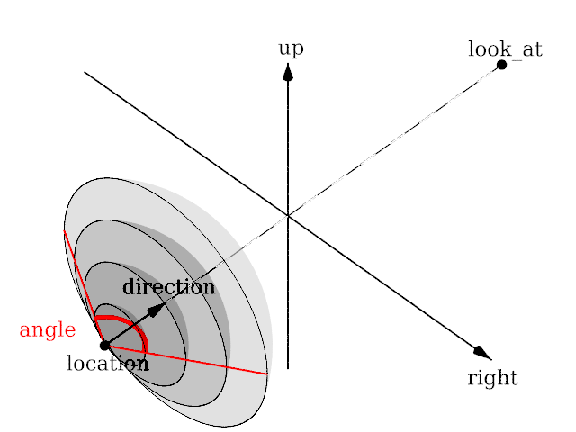
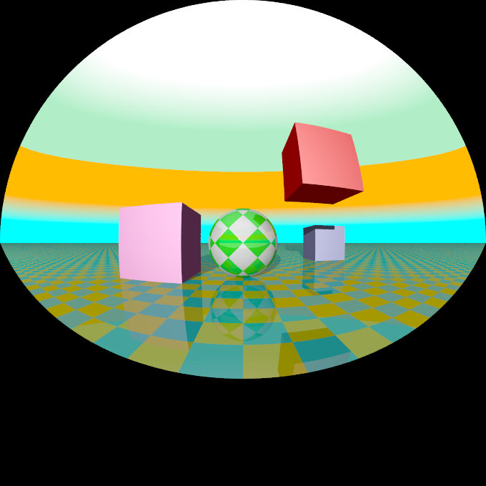
3.4.2.2.4 Fisheye projection
This is a spherical projection. The viewing angle is specified by the angle keyword. An angle of 180 degrees creates the "standard" fisheye while an angle of 360 degrees creates a super-fisheye or "I-see-everything-view". If you use this projection you should get a circular image. If this is not the case, i.e. you get an elliptical image, you should read Aspect Ratio.
|
|
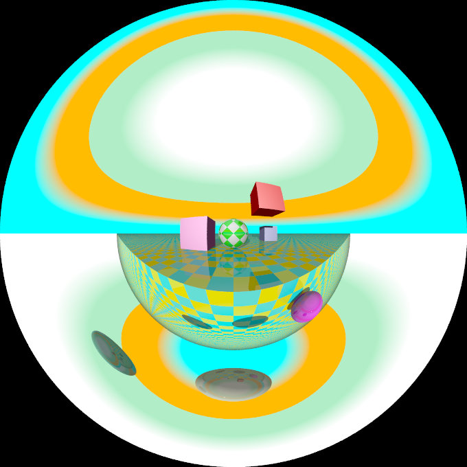
|
The fisheye projection diagram |
A fisheye camera sample image |
Note: The length of the direction, up and right vectors are irrelevant. The angle keyword is the important setting.
3.4.2.2.5 Ultra wide angle projection
The ultra wide angle projection is somewhat similar to the fisheye, but it projects the image onto a rectangle instead of a circle. The viewing angle can be specified by using the angle keyword. The aspect ratio of the lengths of the up/right vectors are used to provide the vertical angle from the horizontal angle, so that the ratio of vertical angle on horizontal angle is identical to the ratio of the length of up on length of right. When the ratio is one, a square is wrapped on a quartic surface defined as follows:
x2+y2+z2 = x2y2 + 1
The section where z=0 is a square, the section where x=0 or y=0 is a circle, and the sections parallel to x=0 or y=0 are ellipses. When the ratio is not one, the bigger angle obviously gets wrapped further. When the angle reaches 180, the border meets the square section. The angle can be greater than 180, in that case, when both (vertical and horizontal) angles are greater than 180, the parts around the corners of the square section will be wrapped more than once. The classical usage (using an angle of 360) but with a up/right ratio of 1/2 up 10*y and right 20*x will keep the top of the image as the zenith, and the bottom of the image as the nadir, avoiding perception issues and giving a full 360 degree view.
|
|
|
The ultra wide angle projection diagram |
An ultra wide angle sample image |
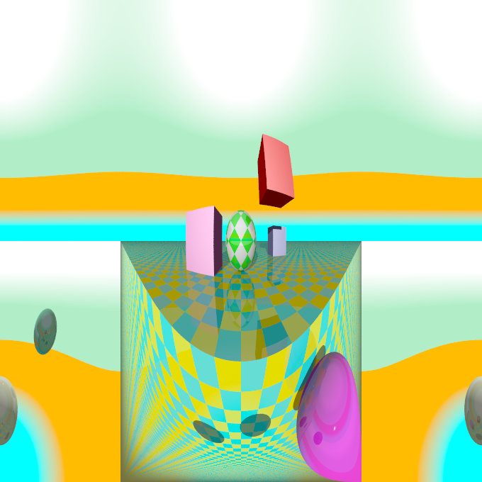
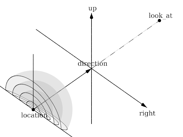
3.4.2.2.6 Omnimax projection
The omnimax projection is a 180 degrees fisheye that has a reduced viewing angle in the vertical direction. In reality this projection is used to make movies that can be viewed in the dome-like Omnimax theaters. The image will look somewhat elliptical.
|
|
|
The omnimax projection diagram |
An omnimax camera sample image |
Note: The use of the angle keyword is irrelevant, the relative length of up and right vectors are what is important.
3.4.2.2.7 Panoramic projection
This projection is called "cylindrical equirectangular projection". It overcomes the degeneration problem of the perspective projection if the viewing angle approaches 180 degrees. It uses a type of cylindrical projection to be able to use viewing angles larger than 180 degrees with a tolerable lateral-stretching distortion. The angle keyword is used to determine the viewing angle.
|
|
|
The panoramic projection diagram |
A panoramic camera sample image |
Note: The angle keyword is irrelevant. The relative length of direction, up and right vectors are important as they define the lengths of the 3 axis of the ellipsoid. With identical length and orthogonal vectors (both strongly recommended, unless used on purpose), it's identical to a spherical camera with angle 180,90.
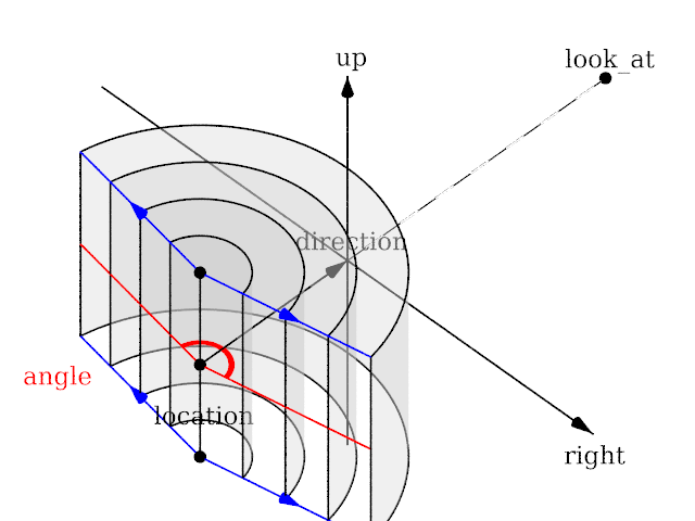
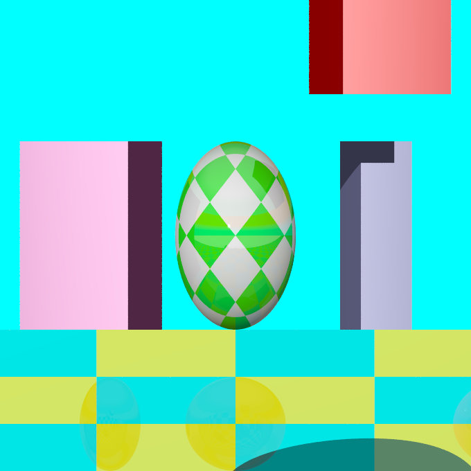
3.4.2.2.8 Cylindrical projection
Using this projection the scene is projected onto a cylinder. There are four different types of cylindrical projections depending on the orientation of the cylinder and the position of the viewpoint. An integer value in the range 1 to 4 must follow the cylinder keyword. The viewing angle and the length of the up or right vector determine the dimensions of the camera and the visible image. The characteristics of different types are as follows:
- vertical cylinder, fixed viewpoint
- horizontal cylinder, fixed viewpoint
- vertical cylinder, viewpoint moves along the cylinder's axis
- horizontal cylinder, viewpoint moves along the cylinder's axis
|
|
|
The type 1 cylindrical projection diagram |
A type 1 cylindrical camera sample image |
|
|
|
The type 2 cylindrical projection diagram |
A type 2 cylindrical camera sample image |
|
|
|
The type 3 cylindrical projection diagram |
A type 3 cylindrical camera sample image |
|
|
|
The type 4 cylindrical projection diagram |
A type 4 cylindrical camera sample image |
3.4.2.2.9 Spherical projection
Using this projection the scene is projected onto a sphere.
The syntax is:
camera {
  spherical
  [angle HORIZONTAL [VERTICAL]]
  [CAMERA_ITEMS...]
  }
The first value after angle sets the horizontal viewing angle of the camera. With the optional second value, the vertical viewing angle is set: both in degrees. If the vertical angle is not specified, it defaults to half the horizontal angle.
The spherical projection is similar to the fisheye projection, in that the scene is projected on a sphere. But unlike the fisheye camera, it uses rectangular coordinates instead of polar coordinates; in this it works the same way as spherical mapping (map_type 1).
This has a number of uses. Firstly, it allows an image rendered with the spherical camera to be mapped on a sphere without distortion (with the fisheye camera, you first have to convert the image from polar to rectangular coordinates in some image editor). Also, it allows effects such as "environment mapping", often used for simulating reflections in scanline renderers.
|
|
|
The spherical projection diagram |
A spherical camera sample image |
Note: The lengths of the direction, up and right vectors are irrelevant. Angle is the important setting, and it gets two values separated by a comma: the first is the horizontal angle, the second is the vertical angle. Both values can reach 360. If the second value is missing, it is set to half the value of the first.
3.4.2.3 Focal Blur
POV-Ray can simulate focal depth-of-field by shooting a number of sample rays from jittered points within each pixel and averaging the results.
To turn on focal blur, you must specify the aperture keyword followed by a float value which determines the depth of the sharpness zone. Large apertures give a lot of blurring, while narrow apertures will give a wide zone of sharpness.
Note: While this behaves as a real camera does, the values for aperture are purely arbitrary and are not related to f-stops.
You must also specify the blur_samples keyword followed by an integer value specifying the maximum number of rays to use for each pixel. More rays give a smoother appearance but is slower. By default no focal blur is used, i. e. the default aperture is 0 and the default number of samples is 0.
The center of the zone of sharpness is specified by the focal_point vector. The zone of sharpness is a plane through the focal_point and is parallel to the camera. Objects close to this plane of focus are in focus and those farther from that plane are more blurred. The default value is focal_point<0,0,0>.
Although blur_samples specifies the maximum number of samples, there is an adaptive mechanism that stops shooting rays when a certain degree of confidence has been reached. At that point, shooting more rays would not result in a significant change.
Extra samples are generated in a circular rather than square pattern when blur_samples is not set to either 4, 7, 19 or 37, leading to a circular rather than square bokeh. The extra samples are generated from a Halton sequence rather than a random stream. You can also optionally specify a minimum number of samples to be taken before testing against the confidence and variance settings. The default is 4, if the blur_samples maximum is less than 7, otherwise the default is 7, to provide a means to get rid of stray non-blurred pixels.
The syntax is:
blur_samples [ MIN_SAMPLES, ] MAX_SAMPLES
The confidence and
variance keywords are followed by float values to control the adaptive function. The confidence value is used to determine when the samples seem to be close enough to the correct color. The variance value specifies an acceptable tolerance on the variance of the samples taken so far. In other words, the process of shooting sample rays is terminated when the estimated color value is very likely (as controlled by the confidence probability) near the real color value.
Since the confidence is a probability its values can range from 0 to less than 1 (the default is 0.9, i. e. 90%). The value for the variance should be in the range of the smallest displayable color difference (the default is 1/128). If 1 is used POV-Ray will issue a warning and then use the default instead.
Rendering with the default settings can result in quite grainy images. This can be improved by using a lower variance. A value of 1/10000 gives a fairly good result (with default confidence and blur_samples set to something like 100) without being unacceptably slow.
Larger confidence values will lead to more samples, slower traces and better images. The same holds for smaller variance thresholds.
Focal blur can also support a user-defined bokeh using the following syntax:
camera {
  // ... focal blur camera definition
  bokeh {
    pigment { ... }
    }
  }
If bokeh is specified, focal blur will use a custom sampling sequence based on the specified pigment's brightness in the range <0,0,0> to <1,1,0> i.e. the unit square in the XY plane.
3.4.2.4 Camera Ray Perturbation
The optional normal may be used to assign a normal pattern to
the camera. For example:
camera{
  location Here
  look_at There
  normal { bumps 0.5 }
  }
All camera rays will be perturbed using this pattern. The image will be distorted as though you were looking through bumpy glass or seeing a reflection off of a bumpy surface. This lets you create special effects. See the animated scene camera2.pov for an example. See Normal for information on normal patterns.
3.4.2.5 Camera Identifiers
Camera identifiers may be declared to make scene files more readable and to parameterize scenes so that changing a single declaration changes many values. You may declare several camera identifiers if you wish. This makes it easy to quickly change cameras. An identifier is declared as follows.
CAMERA_DECLARATION:
  #declare IDENTIFIER = CAMERA |
  #local IDENTIFIER = CAMERA
Where IDENTIFIER is the name of the identifier up to 40 characters long and CAMERA is any valid camera statement. See #declare vs. #local for information on identifier scope. Here is an example...
#declare Long_Lens =
camera {
  location -z*100
  look_at <0,0,0>
  angle 3
  }

#declare Short_Lens =
camera {
  location -z*50
  look_at <0,0,0>
  angle 15
  }

camera {
  Long_Lens  // edit this line to change lenses
  translate <33,2,0>
  }
Note: Only camera transformations can be added to an already declared camera. Camera behaviour changing keywords are not allowed, as they are needed in an earlier stage for resolving the keyword order dependencies.
3.4.3 Atmospheric Effects
Atmospheric effects are a loosely-knit group of features that affect the background and/or the atmosphere enclosing the scene. POV-Ray includes the ability to render a number of atmospheric effects, such as fog, haze, mist, rainbows and skies.
3.4.3.1 Atmospheric Media
Atmospheric effects such as fog, dust, haze, or visible gas may be simulated by a media statement specified in the scene but not attached to any object. All areas not inside a non-hollow object in the entire scene. A very simple approach to add fog to a scene is explained in the section Fog however this kind of fog does not interact with any light sources like media does. It will not show light beams or other effects and is therefore not very realistic.
The atmosphere media effect overcomes some of the fog's limitations by calculating the interaction between light and the particles in the atmosphere using volume sampling. Thus shafts of light beams will become visible and objects will cast shadows onto smoke or fog.
Note: POV-Ray cannot sample media along an infinitely long ray. The ray must be finite in order to be possible to sample. This means that sampling media is only possible for rays that hit an object, so no atmospheric media will show up against the background or sky_sphere. Another way of being able to sample media is using spotlights, because in this case the ray is not infinite, as it is sampled only inside the spotlight cone.
With spotlights you will be able to create the best results because their cone of light will become visible. Pointlights can be used to create effects like street lights in fog. Lights can be made to not interact with the atmosphere by adding media_interaction off to the light source. They can be used to increase the overall light level of the scene to make it look more realistic.
Complete details on media are given in the section Media. Earlier versions of POV-Ray used an atmosphere statement for atmospheric effects but that system was incompatible with the old object halo system. So atmosphere has been eliminated and replaced with a simpler and more powerful media feature. The user now only has to learn one media system for either atmospheric or object use.
If you only want media effects in a particular area, you should use object media rather than only relying upon the media pattern. In general it will be faster and more accurate because it only calculates inside the constraining object.
Note: The atmosphere feature will not work if the camera is inside a non-hollow object (see the section Empty and Solid Objects for a detailed explanation).
3.4.3.2 Background
A background color can be specified if desired. Any ray that does not hit an object will be colored with this color. The default background is black. The syntax for background is:
BACKGROUND:
 background {COLOR}
Note: As of version 3.7 some changes have been made to the way alpha is handled when +ua is activated.
- In previous versions, specifying a background with the
backgroundkeyword would by default supply a background with transmit set to 1.0 (i.e. fully transparent provided that+uais being used). This is no longer the case. While the default background is transparent, any background specified in a scene file (unless 3.6 or earlier compatibility is being used) will now be opaque unless transmit is explicitly given. In other words, usergbft<>rather thanrgb<>in the background statement if you want the old behavior. - The way that objects are blended with the background has changed. Previously the color of the background was not taken into account when calculating effects of transmission through translucent objects when
+uais in effect (i.e. where the background could otherwise have been seen through the object). Now, however, the background color is taken into account, even if it is not otherwise visible. Blending is performed in the same way regardless of the presence of background transparency.
Note: When using Output_Alpha=on or +ua with legacy scenes (the #version directive set to less than 3.7) the background will be suppressed, except in reflections.
3.4.3.3 Fog
If it is not necessary for light beams to interact with atmospheric media,
then fog may be a faster way to simulate haze or fog. This
feature artificially adds color to every pixel based on the distance the ray
has traveled. The syntax for fog is:
FOG:
  fog { [FOG_IDENTIFIER] [FOG_ITEMS...] }
FOG_ITEMS:
  fog_type Fog_Type | distance Distance | COLOR |
  turbulence <Turbulence> | turb_depth Turb_Depth |
  omega Omega | lambda Lambda | octaves Octaves |
  fog_offset Fog_Offset | fog_alt Fog_Alt |
  up <Fog_Up> | TRANSFORMATION
Fog default values:
lambda     : 2.0
fog_type   : 1
fog_offset : 0.0
fog_alt    : 0.0
octaves    : 6
omega      : 0.5
turbulence : <0,0,0>
turb_depth : 0.5
up         : <0,1,0>
Currently there are two fog types, the default fog_type 1 is
a constant fog and fog_type 2 is ground fog. The constant fog
has a constant density everywhere while the ground fog has a constant density
for all heights below a given point on the up axis and thins out along this
axis.
The color of a pixel with an intersection depth d is calculated by
PIXEL_COLOR = exp(-d/D) * OBJECT_COLOR + (1-exp(-d/D)) * FOG_COLOR
where D is the specified value of the required fog distance
keyword. At depth 0 the final color is the object's color. If the
intersection depth equals the fog distance the final color consists of 64%
of the object's color and 36% of the fog's color.
Note: For this equation, a distance of zero is undefined. In practice, povray will treat this value as "fog is off". To use an extremely thick fog, use a small nonzero number such as 1e-6 or 1e-10.
For ground fog, the height below which the fog has constant density is
specified by the fog_offset keyword. The fog_alt
keyword is used to specify the rate by which the fog fades away. The default
values for both are 0.0 so be sure to specify them if ground fog is used. At
an altitude of Fog_Offset+Fog_Alt the fog has a
density of 25%. The density of the fog at height less than or equal to
Fog_Offset is 1.0 and for height larger than than Fog_Offset
is calculated by:
1/(1 + (y - Fog_Offset) / Fog_Alt) ^2
The total density along a ray is calculated by integrating from the height of the starting point to the height of the end point.
The optional up vector specifies a direction pointing up,
generally the same as the camera's up vector. All calculations done
during the ground fog evaluation are done relative to this up vector, i. e.
the actual heights are calculated along this vector. The up vector can also
be modified using any of the known transformations described in
Transformations. Though it may not be a good idea to scale the up
vector - the results are hardly predictable - it is quite useful to be able
to rotate it. You should also note that translations do not affect the up
direction (and thus do not affect the fog).
The required fog color has three purposes. First it defines the color to be used in blending the fog and the background. Second it is used to specify a translucency threshold. By using a transmittance larger than zero one can make sure that at least that amount of light will be seen through the fog. With a transmittance of 0.3 you will see at least 30% of the background. Third it can be used to make a filtering fog. With a filter value larger than zero the amount of background light given by the filter value will be multiplied with the fog color. A filter value of 0.7 will lead to a fog that filters 70% of the background light and leaves 30% unfiltered.
Fogs may be layered. That is, you can apply as many layers of fog as you like. Generally this is most effective if each layer is a ground fog of different color, altitude and with different turbulence values. To use multiple layers of fogs, just add all of them to the scene.
You may optionally stir up the fog by adding turbulence. The turbulence keyword may be followed by a float or vector to specify an amount of turbulence to be used. The omega, lambda and octaves turbulence parameters may also be specified. See the section Turbulence Warp for details on all of these turbulence parameters.
Additionally the fog turbulence may be scaled along the direction of the viewing ray using the turb_depth amount. Typical values are from 0.0 to 1.0 or more. The default value is 0.5 but any float value may be used.
Note: The fog feature will not work if the camera is inside a non-hollow object (see the section Empty and Solid Objects for a detailed explanation).
3.4.3.4 Sky Sphere
The sky sphere is used create a realistic sky background without the need of an additional sphere to simulate the sky. Its syntax is:
SKY_SPHERE:
  sky_sphere { [SKY_SPHERE_IDENTIFIER] [SKY_SPHERE_ITEMS...] }
SKY_SPHERE_ITEM:
  PIGMENT | TRANSFORMATION | [emission]
Note: When using Output_Alpha=on or +ua with legacy scenes (the #version directive set to less than 3.7) the sky_sphere will be suppressed, except in reflections.
The sky sphere can contain several pigment layers with the last pigment being at the top, i. e. it is evaluated last, and the first pigment being at the bottom, i. e. it is evaluated first. If the upper layers contain filtering and/or transmitting components lower layers will shine through. If not lower layers will be invisible.
Note: Version 3.7 changed the effect of filter in a layered-pigment sky_sphere to match the behavior of a corresponding layered-texture large regular sphere. The old behavior, though probably having been unintentional, is automatically re-activated for backward compatibility when a #version of less than 3.7 is specified.
The sky sphere is calculated by using the direction vector as the parameter for evaluating the pigment patterns. This leads to results independent from the view point, which fairly accurately models a real sky, where the distance to the sky is much larger than the distances between visible objects.
Optionally adding the emission keyword allows for brightness tuning of image-mapped sky sphere's. The default is rgb <1,1,1> with higher values increasing the brightness, and lower values correspondingly decrease it. Although primarily intended for easy tuning of light probe skies, the parameter also works with procedural sky pigments.
If you want to add a nice color blend to your background you can easily do this by using the following example.
sky_sphere {
  pigment {
    gradient y
      color_map {
        [ 0.5  color CornflowerBlue ]
        [ 1.0  color MidnightBlue ]
        }
    scale 2
    translate -1
    }
  emission rgb <0.8,0.8,1>
  }
This gives a soft blend from CornflowerBlue at the horizon to MidnightBlue at the zenith. The scale and translate operations are used to map the direction vector values, which lie in the range from <-1, -1, -1> to <1, 1, 1>, onto the range from <0, 0, 0> to <1, 1, 1>. Thus a repetition of the color blend is avoided for parts of the sky below the horizon.
In order to easily animate a sky sphere you can transform it using the usual transformations described in Transformations. Though it may not be a good idea to translate or scale a sky sphere - the results are hardly predictable - it is quite useful to be able to rotate it. In an animation the color blendings of the sky can be made to follow the rising sun for example.
Note: Only one sky sphere can be used in any scene. It also will not work as you might expect if you use camera types like the orthographic or cylindrical camera. The orthographic camera uses parallel rays and thus you will only see a very small part of the sky sphere (you will get one color skies in most cases). Reflections in curved surface will work though, e. g. you will clearly see the sky in a mirrored ball.
3.4.3.5 Rainbow
Rainbows are implemented using fog-like, circular arcs. Their syntax is:
RAINBOW:
  rainbow { [RAINBOW_IDENTIFIER] [RAINBOW_ITEMS...] }
RAINBOW_ITEM:
  direction <Dir> | angle Angle | width Width |
  distance Distance | COLOR_MAP | jitter Jitter | up <Up> |
  arc_angle Arc_Angle | falloff_angle Falloff_Angle
Rainbow default values:
arc_angle     : 180.0
falloff_angle : 180.0
jitter        : 0.0
up            : y
The required direction vector determines the direction of the
(virtual) light that is responsible for the rainbow. Ideally this is an
infinitely far away light source like the sun that emits parallel light rays.
The position and size of the rainbow are specified by the required angle
and width keywords. To understand how they work you should
first know how the rainbow is calculated.
For each ray the angle between the rainbow's direction vector and the
ray's direction vector is calculated. If this angle lies in the interval
from Angle-Width/2 to
Angle+Width/2 the rainbow is hit by the ray. The color is then
determined by using the angle as an index into the rainbow's color_map.
After the color has been determined it will be mixed with the background
color in the same way like it is done for fogs.
Thus the angle and width parameters determine the angles under which the
rainbow will be seen. The optional jitter keyword can be used
to add random noise to the index. This adds some irregularity to the rainbow
that makes it look more realistic.
The required distance keyword is the same like the one used
with fogs. Since the rainbow is a fog-like effect it is possible that the
rainbow is noticeable on objects. If this effect is not wanted it can be
avoided by using a large distance value. By default a sufficiently large
value is used to make sure that this effect does not occur.
The color_map statement is used to assign a color map that
will be mapped onto the rainbow. To be able to create realistic rainbows it
is important to know that the index into the color map increases with the
angle between the ray's and rainbow's direction vector. The index is
zero at the innermost ring and one at the outermost ring. The filter and
transmittance values of the colors in the color map have the same meaning as
the ones used with fogs (see the section Fog).
The default rainbow is a 360 degree arc that looks like a circle. This is no
problem as long as you have a ground plane that hides the lower, non-visible
part of the rainbow. If this is not the case or if you do not want the
full arc to be visible you can use the optional keywords up,
arc_angle and falloff_angle to specify a smaller
arc.
The arc_angle keyword determines the size of the arc in degrees
(from 0 to 360 degrees). A value smaller than 360 degrees results in an arc
that abruptly vanishes. Since this does not look nice you can use the
falloff_angle keyword to specify a region in which the rainbow
will smoothly blend into the background making it vanish softly. The falloff
angle has to be smaller or equal to the arc angle.
The up keyword determines were the zero angle position is. By
changing this vector you can rotate the rainbow about its direction. You
should note that the arc goes from -Arc_Angle/2 to
+Arc_Angle/2. The soft regions go from -Arc_Angle/2 to
-Falloff_Angle/2 and from +Falloff_Angle/2 to
+Arc_Angle/2.
The following example generates a 120 degrees rainbow arc that has a falloff region of 30 degrees at both ends:
rainbow {
  direction <0, 0, 1>
  angle 42.5
  width 5
  distance 1000
  jitter 0.01
  color_map { Rainbow_Color_Map }
  up <0, 1, 0>
  arc_angle 120
  falloff_angle 30
  }
It is possible to use any number of rainbows and to combine them with other atmospheric effects.
3.4.4 Lighting Types
POV-Ray supports several lighting types. The most basic being a highly configurable conventional light source. Scenes can have more than one light source, and light sources can be grouped together with other objects and/or light sources. POV-Ray also supports more sophisticated lighting models such as: global illumination or radiosity and photon mapping.
3.4.4.1 Light Source
The light_source is not really an object. Light sources have no visible shape of their own. They are just points or areas which emit light. They are categorized as objects so that they can be combined with regular objects using union.
Note: Due to a hard-coded limit the number of light sources should not exceed 127. Since the class of the variable that governs this limit is not exclusive to light sources, a value had to be chosen that provides the best balance between performance, memory use and flexibility. See the following news-group discussion for more details and information about ways to overcome this limitation.
The syntax is as follows:
LIGHT_SOURCE:
  light_source {
    <Location>, COLOR
    [LIGHT_MODIFIERS...]
    }
LIGHT_MODIFIER:
  LIGHT_TYPE | SPOTLIGHT_ITEM | AREA_LIGHT_ITEMS |
  GENERAL_LIGHT_MODIFIERS
LIGHT_TYPE:
  spotlight | shadowless | cylinder | parallel
SPOTLIGHT_ITEM:
  radius Radius | falloff Falloff | tightness Tightness |
  point_at <Spot>
PARALLEL_ITEM:
  point_at <Spot>
AREA_LIGHT_ITEM:
  area_light <Axis_1>, <Axis_2>, Size_1, Size_2 |
  adaptive Adaptive | area_illumination [Bool] |
  jitter | circular | orient
GENERAL_LIGHT_MODIFIERS:
  looks_like { OBJECT } |
  TRANSFORMATION fade_distance Fade_Distance |
  fade_power Fade_Power | media_attenuation [Bool] |
  media_interaction [Bool] | projected_through
Light source default values:
LIGHT_TYPE        : pointlight
falloff           : 70
media_interaction : on
media_attenuation : off
point_at          : <0,0,0>
radius            : 70
tightness         : 10
The different types of light sources and the optional modifiers are described in the following sections.
The first two items are common to all light sources. The <Location>
vector gives the location of the light. The COLOR gives the color
of the light. Only the red, green, and blue components are significant. Any
transmit or filter values are ignored.
Note: You vary the intensity of the light as well as the color using this parameter. A color such as
rgb <0.5,0.5,0.5> gives a white light that is half the normal intensity.
All of the keywords or items in the syntax specification above may appear in any order. Some keywords only have effect if specified with other keywords. The keywords are grouped into functional categories to make it clear which keywords work together. The GENERAL_LIGHT_MODIFIERS work with all types of lights and all options.
Note: TRANSFORMATIONS such as translate, rotate etc. may be applied but no other OBJECT_MODIFIERS may be used.
There are three mutually exclusive light types. If no LIGHT_TYPE is
specified it is a point light. The other choices are spotlight
and cylinder.
3.4.4.1.1 Point Lights
The simplest kind of light is a point light. A point light source sends
light of the specified color uniformly in all directions. The default light
type is a point source. The <Location> and
COLOR is all that is required. For example:
light_source {
  <1000,1000,-1000>, rgb <1,0.75,0> //an orange light
  }
3.4.4.1.2 Spotlights
Normally light radiates outward equally in all directions from the source.
However the spotlight keyword can be used to create a cone of
light that is bright in the center and falls of to darkness in a soft fringe
effect at the edge.
Although the cone of light fades to soft edges, objects illuminated by spotlights still cast hard shadows. The syntax is:
SPOTLIGHT_SOURCE:
  light_source {
    <Location>, COLOR spotlight
    [LIGHT_MODIFIERS...]
    }
LIGHT_MODIFIER:
  SPOTLIGHT_ITEM | AREA_LIGHT_ITEMS | GENERAL_LIGHT_MODIFIERS
SPOTLIGHT_ITEM:
  radius Radius | falloff Falloff | tightness Tightness |
  point_at <Spot>
Default values:
radius:    30 degrees
falloff:   45 degrees
tightness:  0
The point_at keyword tells the spotlight to point at a
particular 3D coordinate. A line from the location of the spotlight to the
point_at coordinate forms the center line of the cone of light.
The following illustration will be helpful in understanding how these values
relate to each other.
|
|
The geometry of a spotlight. |
The falloff, radius, and tightness
keywords control the way that light tapers off at the edges of the cone.
These four keywords apply only when the spotlight or
cylinder keywords are used.
The falloff keyword specifies the overall size of the cone of
light. This is the point where the light falls off to zero intensity. The
float value you specify is the angle, in degrees, between the edge of the
cone and center line. The radius keyword specifies the size of
the hot-spot at the center of the cone of light. The
hot-spot is a brighter cone of light inside the spotlight cone
and has the same center line. The radius value specifies the
angle, in degrees, between the edge of this bright, inner cone and the center
line. The light inside the inner cone is of uniform intensity. The light
between the inner and outer cones tapers off to zero.
For example, assuming a tightness 0, with radius 10 and falloff 20 the light
from the center line out to 10 degrees is full intensity. From 10 to 20
degrees from the center line the light falls off to zero intensity. At 20
degrees or greater there is no light.
Note: If the radius and falloff values are close or equal the light intensity drops rapidly and the spotlight has a sharp edge.
The values for the radius, and tightness parameters are half the opening angles of the
corresponding cones, both angles have to be smaller than 90 degrees. The
light smoothly falls off between the radius and the falloff angle like shown
in the figures below (as long as the radius angle is not negative).
|
|
Intensity multiplier curve with a fixed falloff angle of 45 degrees. |
|
|
Intensity multiplier curve with a fixed radius angle of 45 degrees. |
The tightness keyword is used to specify an
additional exponential softening of the edges. A value other than 0, will
affect light within the radius cone as well as light in the falloff cone.
The intensity of light at an angle from the center line is given by:
intensity * cos(angle)tightness.
The default value for tightness is 0. Lower
tightness values will make the spotlight brighter, making the spot wider and
the edges sharper. Higher values will dim the spotlight, making the spot
tighter and the edges softer. Values from 0 to 100 are acceptable.
|
|
Intensity multiplier curve with fixed angle and falloff angles of 30 and 60 degrees respectively and different tightness values. |
You should note from the figures that the radius and falloff angles interact with the tightness parameter. To give the tightness value full control over the spotlight's appearance use radius 0 falloff 90. As you can see from the figure below. In that case the falloff angle has no effect and the lit area is only determined by the tightness parameter.
|
|
Intensity multiplier curve with a negative radius angle and different tightness values. |
Spotlights may be used any place that a normal light source is used. Like any light sources, they are invisible. They may also be used in conjunction with area lights.
3.4.4.1.3 Cylindrical Lights
The cylinder keyword specifies a cylindrical light source
that is great for simulating laser beams. Cylindrical light sources work
pretty much like spotlights except that the light rays are constrained by a
cylinder and not a cone. The syntax is:
CYLINDER_LIGHT_SOURCE:
  light_source {
    <Location>, COLOR cylinder
    [LIGHT_MODIFIERS...]
    }
LIGHT_MODIFIER:
  SPOTLIGHT_ITEM | AREA_LIGHT_ITEMS | GENERAL_LIGHT_MODIFIERS
SPOTLIGHT_ITEM:
  radius Radius | falloff Falloff | tightness Tightness |
  point_at <Spot>
Default values:
radius:     0.75 degrees
falloff:    1    degrees
tightness:  0
The point_at, radius, falloff and
tightness keywords control the same features as with the
spotlight. See Spotlights for details.
You should keep in mind that the cylindrical light source is still a point light source. The rays are emitted from one point and are only constraint by a cylinder. The light rays are not parallel.
3.4.4.1.4 Parallel Lights
syntax:

light_source {
  LOCATION_VECTOR, COLOR
  [LIGHT_SOURCE_ITEMS...]
  parallel
  point_at VECTOR
  }
The parallel keyword can be used with any type of light source.
Note: For normal point lights, point_at must come after
parallel.
Parallel lights are useful for simulating very distant light sources, such as sunlight. As the name suggests, it makes the light rays parallel.
Technically this is done by shooting rays from the closest point on a plane to the
object intersection point. The plane is determined by a perpendicular defined by the
light location and the point_at vector.
Two things must be considered when choosing the light location (specifically, its distance):
- Any parts of an object above the light plane still get illuminated according to the light direction, but they will not cast or receive shadows.
fade_distanceandfade_poweruse the lightlocationto determine distance for light attenuation, so the attenuation still looks like that of a point source.
Area light also uses the light location in its calculations.
3.4.4.1.5 Area Lights
Area light sources occupy a finite, one or two-dimensional area of space. They can cast soft shadows because an object can partially block their light. Point sources are either totally blocked or not blocked.
The area_light keyword in POV-Ray creates sources that are rectangular in shape, sort of like a flat panel light. Rather than performing the complex calculations that would be required to model a true area light, it is approximated as an array of point light sources spread out over the area occupied by the light. The array-effect applies to shadows only, however with the addition of the area_illumination keyword, full area light diffuse and specular illumination can be achieved. The object's illumination is still that of a point source. The intensity of each individual point light in the array is dimmed so that the total amount of light emitted by the light is equal to the light color specified in the declaration. The syntax is:
AREA_LIGHT_SOURCE:
  light_source {
    LOCATION_VECTOR, COLOR
    area_light
    AXIS_1_VECTOR, AXIS_2_VECTOR, Size_1, Size_2
    [ adaptive Adaptive ] [ area_illumination on/off ]
    [ jitter ] [ circular ] [ orient ]
    [ [LIGHT_MODIFIERS...]
    }
Any type of light source may be an area light.
The area_light keyword defines the location, the size and orientation of the area light as well as the number of lights in the light source array. The location vector is the centre of a rectangle defined by the two vectors <Axis_1> and <Axis_2>. These specify the lengths and directions of the edges of the light.
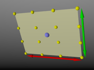
|
|
4x4 Area light, location and vectors. |
Since the area lights are rectangular in shape these vectors should be perpendicular to each other. The larger the size of the light the thicker the soft part of shadows will be. The integers Size_1 and Size_2 specify the number of rows and columns of point sources of the. The more lights you use the smoother the shadows, but render time will increase.
Note: It is possible to specify spotlight parameters along with the area light parameters to create area spotlights. Using area spotlights is a good way to speed up scenes that use area lights since you can confine the lengthy soft shadow calculations to only the parts of your scene that need them.
An interesting effect can be created using a linear light source. Rather than having a rectangular shape, a linear light stretches along a line sort of like a thin fluorescent tube. To create a linear light just create an area light with one of the array dimensions set to 1.
Note: In version 3.7 experimental support for full area light diffuse and specular illumination was added.
This feature is off by default, so area lights will work as previously expected, and can be turned on by specifying the area_illumination keyword, followed by the optional on/off keyword, in the light source definition. As with area lights, the Size_1 and Size_2 parameters determine the quality of the lighting, as well as the quality of the shadows.
The jitter keyword is optional. When used it causes the positions of the point lights in the array to be randomly jittered to eliminate any shadow banding that may occur. The jittering is completely random from render to render and should not be used when generating animations.
The adaptive keyword is used to enable adaptive sampling of the light source. By default POV-Ray calculates the amount of light that reaches a surface from an area light by shooting a test ray at every point light within the array. As you can imagine this is very slow. Adaptive sampling on the other hand attempts to approximate the same calculation by using a minimum number of test rays. The number specified after the keyword controls how much adaptive sampling is used. The higher the number the more accurate your shadows will be but the longer they will take to render. If you are not sure what value to use a good starting point is adaptive 1. The adaptive keyword only accepts integer values and cannot be set lower than 0.
When performing adaptive sampling POV-Ray starts by shooting a test ray at each of the four corners of the area light. If the amount of light received from all four corners is approximately the same then the area light is assumed to be either fully in view or fully blocked. The light intensity is then calculated as the average intensity of the light received from the four corners. However, if the light intensity from the four corners differs significantly then the area light is partially blocked. The area light is split into four quarters and each section is sampled as described above. This allows POV-Ray to rapidly approximate how much of the area light is in view without having to shoot a test ray at every light in the array. Visually the sampling goes like shown below.
|
|
Area light adaptive samples. |
While the adaptive sampling method is fast (relatively speaking) it can sometimes produce inaccurate shadows. The solution is to reduce the amount of adaptive sampling without completely turning it off. The number after the adaptive keyword adjusts the number of times that the area light will be split before the adaptive phase begins. For example if you use adaptive 0 a minimum of 4 rays will be shot at the light. If you use adaptive 1 a minimum of 9 rays will be shot (adaptive
2 gives 25 rays, adaptive 3 gives 81 rays, etc). Obviously the more shadow rays you shoot the slower the rendering will be so you should use the lowest value that gives acceptable results.
The number of rays never exceeds the values you specify for rows and columns of points. For example area_light x,y,4,4 specifies a 4 by 4 array of lights. If you specify adaptive 3 it would mean that you should start with a 9 by 9 array. In this case no adaptive sampling is done. The 4 by 4 array is used.
The circular keyword has been added to area lights in order to better create circular soft shadows. With ordinary area lights the pseudo-lights are arranged in a rectangular grid and thus project partly rectangular shadows around all objects, including circular objects. By including the circular tag in an area light, the light is stretched and squashed so that it looks like a circle: this way, circular or spherical light sources are better simulated.
A few things to remember:
- Circular area lights can be ellipses: the AXIS_1_VECTOR and AXIS_2_VECTOR define the shape and orientation of the circle; if the vectors are not equal, the light source is elliptical in shape.
- Rectangular artefacts may still show up with very large area grids.
- There is no point in using
circularwith linear area lights or area lights which have a 2x2 size. - The area of a circular light is roughly 78.5 per cent of a similar size rectangular area light. Increase your axis vectors accordingly if you wish to keep the light source area constant.
The orient keyword has been added to area lights in order to better create soft shadows. Without this modifier, you have to take care when choosing the axis vectors of an area_light, since they define both its area and orientation. Area lights are two dimensional: shadows facing the area light receive light from a larger surface area than shadows at the sides of the area light.
|
|
Area light facing object. |
Actually, the area from which light is emitted at the sides of the area light is reduced to a single line, only casting soft shadows in one direction.
|
|
Area light not facing object. |
Between these two extremes the surface area emitting light progresses gradually. By including the orient modifier in an area light, the light is rotated so that for every shadow test, it always faces the point being tested. The initial orientation is no longer important, so you only have to consider the desired dimensions (area) of the light source when specifying the axis vectors. In effect, this makes the area light source appear 3-dimensional (e.g. an area_light with perpendicular axis vectors of the same size and dimensions using circular and orient simulates a spherical light source).
Orient has a few restrictions:
- It can be used with circular lights only.
- The two axes of the area light must be of equal length.
- The two axes of the area light should use an equal number of samples, and that number should be greater than one
These three rules exist because without them, you can get unpredictable results from the orient feature.
If one of the first two rules is broken, POV-Ray will issue a warning and correct the problem. If the third rule is broken, you will only get the error message, and POV-Ray will not automatically correct the problem.
3.4.4.1.6 Shadowless Lights
Using the shadowless keyword you can stop a light source from
casting shadows. These lights are sometimes called fill lights.
They are another way to simulate ambient light however shadowless lights have
a definite source. The syntax is:
SHADOWLESS_LIGHT_SOURCE:
  light_source {
    <Location>, COLOR shadowless
    [LIGHT_MODIFIERS...]
    }
LIGHT_MODIFIER:
  AREA_LIGHT_ITEMS | GENERAL_LIGHT_MODIFIERS
shadowless may be used with all types of light sources.
The only restriction is that shadowless should be before or
after all spotlight or cylinder option keywords. Do not mix or you get
the message Keyword 'the one following shadowless' cannot be used with
standard light source. Also note that shadowless lights will not cause
highlights on the illuminated objects.
3.4.4.1.7 Looks_like
Normally the light source itself has no visible shape. The light simply
radiates from an invisible point or area. You may give a light source any
shape by adding a looks_like { OBJECT }
statement.
There is an implied no_shadow attached to the
looks_like object so that light is not blocked by the object. Without
the automatic no_shadow the light inside the object would not
escape. The object would, in effect, cast a shadow over everything.
If you want the attached object to block light then you should attach it
with a union and not a looks_like as follows:
union {
  light_source { <100, 200, -300> color White }
  object { My_Lamp_Shape }
  }
Presumably parts of the lamp shade are transparent to let some light out.
3.4.4.1.8 Projected_Through
Syntax:
light_source {
  LOCATION_VECTOR, COLOR
  [LIGHT_SOURCE_ITEMS...]
  projected_through { OBJECT }
  }
Projected_through can be used with any type of light source. Any object can be
used, provided it has been declared before.
Projecting a light through an object can be thought of as the opposite of
shadowing: only the light rays that hit the projected_through object
will contribute to the scene.
This also works with area_lights, producing spots of light with soft edges.
Any objects between the light and the projected through object will not cast
shadows for this light. Also any surface within the projected through object
will not cast shadows.
Any textures or interiors on the object will be stripped and the object will not
show up in the scene.
3.4.4.1.9 Light Fading
By default POV-Ray does not diminish light from any light source as it
travels through space. In order to get a more realistic effect
fade_distance and fade_power keywords followed by float
values can be used to model the distance based falloff in light
intensity.
The fade_distance is used to specify the distance at which the full light intensity arrives, i.e.: the intensity which was given by the color attribute. The actual attenuation is described by the fade_power keyword, which determines the falloff rate. For example linear or quadratic falloff can be used by setting the fade_power to 1 or 2 respectively.
The complete formula to calculate the factor by which the light is attenuated is:
|
|
The attenuation of light fading formula |
Where d is the distance the light has traveled.
|
|
Light fading functions for different fading powers |
With any given value for fade_distance, either larger OR smaller than one, the light intensity at distances smaller than that given value actually increases. The internal calculation used to determine the attenuation factor is set up in a way so that one could set the fade distance and know that for any given fade distance, the light value would equal the set intensity. Lastly, only light coming directly from light sources is attenuated, and that reflected or refracted light is not attenuated by distance.
However, further investigation does reveal certain short comings with this method, as it doesn't follow a very good inverse-squared relationship over the fade distance and somewhat beyond. In other words, the function does break down to be very close to inverse squared as the distance from the given value for fade_distance gets significantly larger.
To that end consider the following:
A value for the light source intensity can be easily calculated when you take into account the distance from the light source to the scene center, or the object to be illuminated, and you set a relatively small value for fade_distance e.g.: the size of the light itself, relative to the scene dimensions.
The following example, that takes the inverse of the above formula that was used to calculate the factor by which the light is attenuated.
// setup the function
#declare Intensity_Factor = function (LD,FD,FP) {pow(1+(LD/FD),FP)/2};

// the translated position of the light source
#declare Light_Position = <0,0,-2400>;

// determine the light distance
#declare Light_Distance = vlength(Light_Position-<0,0,0>);

// scaled size of the light source
#declare Fade_Distance = 4.5;

// linear (1) or quadratic (2) falloff
#declare Fade_Power = 2;
Note: The above example calculates Light_Distance to the scene center, but you could have just as easily used the location of an object.
Now all you have to do is setup the light source. The #debug statements make it easy to see whats going on while tuning the light source.
#debug concat ("\nFade Distance: ", str(Fade_Distance,2,4))
#debug concat ("\nLight Distance: ", str(Light_Distance,5,4)," \n")
#debug concat ("Intensity Factor: ", str(Intensity_Factor (Light_Distance, Fade_Distance, Fade_Power),6,4)
#debug concat ("\n\n")

light_source {
  0, rgb <0.9,0.9,1> * Intensity_Factor (Light_Distance, Fade_Distance, Fade_Power)
  fade_distance Fade_Distance
  fade_power Fade_Power
  translate Light_Position
  }
At first glance this may seem counter-intuitive but it works out well given the small value used for Fade_Distance. You should be aware that this method is meant to give a light strength value of ONE at the point of interest ONLY. In other words, the point represented by the calculated value Light_Distance in the above example. Naturally objects closer to the light source will get a stronger illumination, while objects further away will receive less.
3.4.4.1.10 Atmospheric Media Interaction
By default light sources will interact with an atmosphere added to the
scene. This behavior can be switched off by using media_interaction off
inside the light source statement.
Note: In POV-Ray 3.0 this feature was turned off
and on with the atmosphere keyword.
3.4.4.1.11 Atmospheric Attenuation
Normally light coming from light sources is not influenced by fog or
atmospheric media. This can be changed by turning the media_attenuation on
for a given light source on. All light coming from this light source will now
be diminished as it travels through the fog or media. This results in an
distance-based, exponential intensity falloff ruled by the used fog or media.
If there is no fog or media no change will be seen.
Note: In POV-Ray 3.0 this
feature was turned off and on with the atmospheric_attenuation keyword.
3.4.4.2 Light Group
Light groups make it possible to create a union of light sources and objects, where the objects in the group are illuminated by the lights in the group or, if so desired, by the global light sources as well. The light sources in the group can only illuminate the objects that are in the group, this also applies to scattering media, and it must be included in the light group as well. Keep in mind that if the scattering media also has an absorption component, it will be affected by light sources that are not in the light group definition.
Light groups are for example useful when creating scenes in which some objects turn out to be too dark but the average light is exactly how it should be, as the light sources in the group do not contribute to the global lighting.
Syntax :
light_group {
  LIGHT_GROUP LIGHT  |
  LIGHT_GROUP OBJECT |
  LIGHT_GROUP
  [LIGHT_GROUP MODIFIER]
  }

LIGHT_GROUP LIGHT:
  light_source | light_source IDENTIFIER
LIGHT_GROUP OBJECT:
  OBJECT | OBJECT IDENTIFIER
LIGHT_GROUP MODIFIER:
  global_lights BOOL | TRANSFORMATION
- To illuminate objects in the group with the light from global light sources, add
global_lights onto the light group definition. - Light groups may be nested. In this case light groups inherit the light sources of the light group in which they are contained.
- Light groups can be seen as a
unionof an object with alight_sourceand can be used with CSG.
Some examples of a simple light group:
#declare RedLight =
light_source {
  <-500,500,-500>
  rgb <1,0,0>
  }

light_group {
  light_source {RedLight}
  sphere {0,1 pigment {rgb 1}}
  global_lights off
  }
A nested light group:
#declare L1 =
light_group {
  light_source {<10,10,0>, rgb <1,0,0>}
  light_source {<0,0,-100>, rgb <0,0,1>}
  sphere {0,1 pigment {rgb 1}}
  }

light_group {
  light_source {<0,100,0>, rgb 0.5}
  light_group {L1}
  }
Light groups with CSG:
difference {
  light_group {
    sphere {0,1 pigment {rgb 1}}
    light_source {<-100,0,-100> rgb <1,0,0>}
    global_lights off
    }
  light_group {
    sphere {<0,1,0>,1 pigment {rgb 1}}
    light_source {<100,100,0> rgb <0,0,1>}
    global_lights off
    }
  rotate <-45,0,0>
  }
In the last example the result will be a sphere illuminated red, where the part that is differenced away is illuminated blue. The end result is comparable to the difference between two spheres with a different pigment.
3.4.4.3 Radiosity
3.4.4.3.1 Radiosity Basics
Radiosity is an extra calculation that more realistically computes the diffuse inter-reflection of light. This diffuse inter-reflection can be seen if you place a white chair in a room full of blue carpet, blue walls and blue curtains. The chair will pick up a blue tint from light reflecting off of other parts of the room. Also notice that the shadowed areas of your surroundings are not totally dark even if no light source shines directly on the surface. Diffuse light reflecting off of other objects fills in the shadows. Typically ray-tracing uses a trick called ambient light to simulate such effects but it is not very accurate.
Radiosity calculations are only made when a radiosity{} block is used inside the global_settings{} block.
The following sections describes how radiosity works, how to control it with various global settings and tips on trading quality vs. speed.
3.4.4.3.2 How Radiosity Works
The problem of ray-tracing is to figure out what the light level is at each point that you can see in a scene. Traditionally, in ray tracing, this is broken into the sum of these components:
- Diffuse
- the effect that makes the side of things facing the light brighter;
- Specular
- the effect that makes shiny things have dings or sparkles on them;
- Reflection
- the effect that mirrors give; and
- Ambient
- the general all-over light level that any scene has, which keeps things in shadow from being pure black.
POV-Ray's radiosity system, based on a method by Greg Ward, provides a way to replace the last term - the constant ambient light value - with a light level which is based on what surfaces are nearby and how bright in turn they are.
The first thing you might notice about this definition is that it is circular: the brightness and color of everything is dependent on everything else and vice versa. This is true in real life but in the world of ray-tracing, we can make an approximation. The approximation that is used is: the objects you are looking at have their ambient values calculated for you by
checking the other objects nearby. When those objects are checked during this process, however, their diffuse term is used. The brightness of radiosity in POV-Ray is based on two things:
- the amount of light gathered
- the diffuse property of the surface finish
Note: The following is an important behavior change!
Previously an object could have both radiosity and an ambient term. This is no longer the case, as when radiosity is used an objects ambient term is effectively set to zero. See the emission keyword that has been added to the finish block if the intent is to model a glowing object.
How does POV-Ray calculate the ambient term for each point? By sending out more rays, in many different directions, and averaging the results. A typical point might use 200 or more rays to calculate its ambient light level correctly.
Now this sounds like it would make the ray-tracer 200 times slower. This is true, except that the software takes advantage of the fact that ambient light levels change quite slowly (remember, shadows are calculated separately, so sharp shadow edges are not a problem). Therefore, these extra rays are sent out only once in a while (about 1 time in 50), then these calculated values are saved and reused for nearby pixels in the image when possible.
This process of saving and reusing values is what causes the need for a variety of tuning parameters, so you can get the scene to look just the way you want.
3.4.4.3.3 Adjusting Radiosity
As described earlier, radiosity is turned on by using the radiosity{} block in global_setting.
Radiosity has many parameters that are specified as follows:
global_settings { radiosity { [RADIOSITY_ITEMS...] } }
RADIOSITY_ITEMS:
  adc_bailout Float | always_sample Bool | brightness Float |
  count Integer [,Integer] | error_bound Float | gray_threshold Float |
  low_error_factor Float | max_sample Float | media Bool |
  maximum_reuse Float | minimum_reuse Float | nearest_count Integer [,Integer] |
  normal Bool | pretrace_start Float |
  pretrace_end Float | recursion_limit Integer | subsurface Bool
Each item is optional and may appear in any order. If an item is specified more than once the last setting overrides previous values. Details on each item is given in the following sections.
Note: Considerable changes have been made to the way radiosity works in POV-Ray 3.7
compared to previous versions. Old scenes will not render with exactly the same results. It is not possible to use the #version directive to get backward compatibility for radiosity.
3.4.4.3.3.1 adc_bailout
You can specify an adc_bailout for radiosity rays. Usually the default of 0.01 will give good results, but for scenes with bright emissive objects it should be set to adc_bailout = 0.01 / brightest_emissive_object.
3.4.4.3.3.2 always_sample
Since always_sample off is the default, POV-Ray will only use the data from the pretrace step and not gather any new samples during the final radiosity pass. This produces higher quality results, and quicker renders. It may also reduce the splotchy appearance of the radiosity samples, and can be very useful when reusing previously saved radiosity data. If you find the need to override the behavior, you can do so by specifying always_sample on.
3.4.4.3.3.3 brightness
The brightness keyword specifies a float value that is the degree to which objects are brightened before being returned upwards to the rest of the system. Ideally brightness should be set to the default value of 1.0. If the overall brightness doesn't seem to fit, the diffuse color of objects and/or the overall brightness of light sources (including emission > 0 objects) should be adjusted.
As an example, a typical problem encountered in radiosity scenes is, when setting pigment {rgb 1} and diffuse 1.0, then tweaking the light source(s) and ambient_light setting to make the image look right. It just doesn't work properly in radiosity scenes, as it will give too strong inter-reflections. While you can compensate for this by reducing radiosity brightness, it's generally discouraged. In this case the surface properties should be fixed (e.g. diffuse set to something around 0.7, which is much more realistic).
An exception, calling for the adjustment of radiosity brightness, would be to compensate for a low recursion_limit setting (e.g recursion_limit 1). In such a case, increasing brightness will help maintain a realistic overall brightness.
3.4.4.3.3.4 count
The integer number of rays that are sent out whenever a new radiosity value has to be calculated is given by count. The default value is 35, if the value exceeds 1600, POV-Ray will use a Halton sequence instead of the default built-in sequence. When this value is too low, the light level will tend to look a little bit blotchy, as if the surfaces you are looking at were slightly warped. If this is not important to your scene (as in the case that you have a bump map or if you have a strong texture) then by all means use a lower number.
By default, POV-Ray uses the same set of directions for each new radiosity value to calculate. In order to cover more directions in total without increasing the number of rays to trace, count accepts an optional second parameter which specifies the total number of directions from which to choose. POV-Ray will then draw directions from this pool in a round-robin fashion.
3.4.4.3.3.5 error_bound
The error_bound float value is one of the two main speed/quality tuning values (the other is of course the number of rays shot). In an ideal world, this would be the only value needed. It is intended to mean the fraction of error tolerated. For example, if it were set to 1 the algorithm would not calculate a new value until the error on the last one was estimated at as high as 100%. Ignoring the error introduced by rotation for the moment, on flat surfaces this is equal to the fraction of the reuse distance, which in turn is the distance to the closest item hit. If you have an old sample on the floor 10 inches from a wall, an error bound of 0.5 will get you a new sample at a distance of about 5 inches from the wall.
The default value of 1.8 is good for a smooth general lighting effect. Using lower values is more accurate, but it will strongly increase the danger of artifacts and therefore require higher count. You can use values even lower than 0.1 but both render time and memory use can become extremely high.
3.4.4.3.3.6 gray_threshold
Diffusely inter-reflected light is a function of the objects around the point in question. Since this is recursively defined to millions of levels of recursion, in any real life scene, every point is illuminated at least in part by every other part of the scene. Since we cannot afford to compute this, if we only do one bounce, the calculated ambient light is very strongly affected by the colors of the objects near it. This is known as color bleed and it really happens but not as much as this calculation method would have you believe. The gray_threshold float value grays it down a little, to make your scene more believable. A value of .6 means to calculate the ambient value as 60% of the equivalent gray value calculated, plus 40% of the actual value calculated. At 0%, this feature does nothing. At 100%, you always get white/gray ambient light, with no hue.
Note: This does not change the lightness/darkness, only the strength of hue/grayness (in HLS terms, it changes S only). The default value is 0.0
3.4.4.3.3.7 low_error_factor
If you calculate just enough samples, but no more, you will get an image which has slightly blotchy lighting. What you want is just a few extra interspersed, so that the blending will be nice and smooth. The solution to this is the mosaic preview, controlled by
pretrace, it goes over the image one or more times beforehand, calculating radiosity values. To ensure that you get a few extra, the radiosity algorithm lowers the error bound during the pre-final passes, then sets it back just before the final pass. The low_error_factor is a float tuning value which sets the amount that the error bound is dropped during the preliminary image passes. If your low error factor is 0.8 and your error bound is set to 0.4 it will really use an error bound of 0.32 during the first passes and 0.4 on the final pass. The default value is 0.5.
3.4.4.3.3.8 max_sample
Sometimes there can be splotchy patches that are caused by objects that are very bright. This can be sometimes avoided by using the max_sample keyword. max_sample takes a float parameter which specifies the brightest that any gathered sample is allowed to be. Any samples brighter than this will have their brightness decreased (without affecting color). Note however that this mechanism will somewhat darken the overall brightness in an unrealistic way. Specifying a non-positive value for max_sample will allow any brightness of samples (which is the default).
3.4.4.3.3.9 maximum_reuse
The maximum_reuse parameter works in conjunction with, and is similar to that of minimum_reuse, the only difference being that it is an upper bound rather than a lower one. The default value is 0.200.
Note: If you choose to adjust either the minimum_reuse or maximum_reuse settings they are subject to the criteria listed below:
- If
minimum_reuse > maximum_reuse/2with only one value is specified, a warning is issued and the unspecified value is adjusted. - If
minimum_reuse > maximum_reuse/2with both values specified, a warning is issued and neither value is modified. - If
minimum_reuse >= maximum_reuse, an error is generated.
3.4.4.3.3.10 minimum_reuse
The minimum effective radius ratio is set by minimum_reuse float value. This is the fraction of the screen width which sets the minimum radius of reuse for each sample point (actually, it is the fraction of the distance from the eye but the two are roughly equal for normal camera angles). For example, if the value is 0.02, the radius of maximum reuse for every sample is set to whatever ground distance corresponds to 2% of the width of the screen. Imagine you sent a ray off to the horizon and it hits the ground at a distance of 100 miles from your eye point. The reuse distance for that sample will be set to 2 miles. At a resolution of 300*400 this will correspond to (very roughly) 8 pixels. The theory is that you do not want to calculate values for every pixel into every crevice everywhere in the scene, it will take too long. This sets a minimum bound for the reuse. If this value is too low, (which it should be in theory) rendering gets slow, and inside corners can get a little grainy. If it is set too high, you do not get the natural darkening of illumination near inside edges, since it reuses. At values higher than 2% you start getting more just plain errors, like reusing the illumination of the open table underneath the apple. Remember that this is a unit less ratio. The default value is 0.015.
3.4.4.3.3.11 nearest_count
The nearest_count integer value is the minimum number of old radiosity values blended together to create a new interpolated value. There is no upper limit on the number of samples blended, all available samples are blended that match the error_bound and maximum_reuse settings. When an optional second parameter (adaptive radiosity pretrace) is specified after the nearest_count keyword, pretrace will stop re-iterating over areas where, on average, that many average-quality samples are already present per ray. (The actual number of samples required to satisfy the nearest_count settings is influenced by sample quality, with high-quality samples reducing the effective number of samples required, down to 1/4 of the parameter value in extreme cases, and low-quality samples increasing the number.) With a setting lower than 4, things can get pretty patchy, this can be useful for debugging. Conversely, the nearest_count upper limit setting is 20, since values greater than 20 are not very useful in practice, and that is currently the size of the array allocated. The default value is 5.
3.4.4.3.3.12 pretrace_start and pretrace_end
To control the radiosity pre-trace gathering step, use the keywords pretrace_start and pretrace_end. Each of these is followed by a decimal value between 0.0 and 1.0 which specifies the size of the blocks in the mosaic preview as a percentage of the image size. The defaults are 0.08 for pretrace_start and 0.04 for pretrace_end.
3.4.4.3.3.13 recursion_limit
The recursion_limit is an integer value which determines how many recursion levels are used to calculate the diffuse inter-reflection. The default value is 2, the upper limit is 20. In practice, values greater than 3 are seldom useful.
3.4.4.3.4 Configuring Radiosity
The following parameters deal with configuring radiosity and how it interacts with other features. See also these additional command line options for more control.
3.4.4.3.4.1 Importance
If you have some comparatively small yet bright objects in your scene, radiosity will tend to produce bright splotchy artifacts unless you use a pretty high number of rays, which in turn will tremendously increase rendering time. To somewhat mitigate this issue, full ray computations are performed only for a certain portion of sample rays, depending on the ''importance'' of the first object each ray encounters. Importance can be assigned on a per-object basis using the following syntax:
sphere { ... radiosity { importance IMPORTANCE } }
Where IMPORTANCE is a value in the range of greater than 0.0 to less than or equal to 1.0 specifying the percentage of rays to actually compute on average. A particular ray will only be fully computed if it is within the first COUNT*IMPORTANCE rays of the sampling sequence; due to the low-discrepancy sub-random nature of the sequence, this is mostly equivalent to a per-ray weighted random choice, while maintaining a low-discrepancy uniform distribution on a per-object basis. Rays actually computed are weighted to compensate for those not computed.
Objects derived from previously defined objects will default to the inherited importance. CSG components without an explicit importance value set will default to their parent object's importance. Other objects will normally default to importance 1.0, however this can be changed in a default{} block:
default { radiosity { importance DEFAULT_IMPORTANCE } }
3.4.4.3.4.2 Media and Radiosity
Radiosity estimation can be affected by media. To enable this feature, add media on to the radiosity{} block. The default is off
3.4.4.3.4.3 No Radiosity
Specifying no_radiosity in an object block makes that object invisible to radiosity rays, in the same way as no_image, no_reflection and no_shadow make an object invisible to primary, reflected and shadow test rays, respectively.
3.4.4.3.4.4 Normal and Radiosity
Radiosity estimation can be affected by normals. To enable this feature, add normal on to the radiosity{} block. The default is off
3.4.4.3.4.5 Save and Load Radiosity Data
In general, it is not a good idea to save and load radiosity data if scene objects are moving. Even after the data is loaded, more samples may be taken during the final rendering phase, particularly if you've specified always_sample on.
Note: The method to load and save radiosity data has been changed to a command line option. See section radiosity load and save for more details.
3.4.4.3.4.6 Subsurface and Radiosity
To specify whether radiosity sampling should honor subsurface light transport, you should place the following in the global settings radiosity block:
  global_settings {
    radiosity { subsurface BOOL }
    }
If this setting is off, the default, radiosity based diffuse illumination is computed as if the surrounding objects had subsurface light transport turned off. Setting this to on may improve realism especially in the presence of materials with high translucency, but at some cost in rendering time.
See the section Subsurface Light Transport for more information about the role of subsurface in the global settings block.
3.4.4.3.5 Tips on Radiosity
Have a look at the Radiosity Tutorial to get a feel for what the visual result of changing radiosity parameters is.
If you want to see where your values are being calculated set radiosity count down to about 20, set radiosity nearest_count to 1 and set gray_threshold to 0. This will make everything maximally patchy, so you will be able to see the borders between patches. There will have been a radiosity calculation at the center of most patches. As a bonus, this is quick to run. You can then change the error_bound up and down to see how it changes things. Likewise
modify minimum_reuse.
One way to get extra smooth results: crank up the sample count (we have gone as high as 1300) and drop the low_error_factor to something small like 0.6. Bump up the nearest_count to 7 or 8. This will get better values, and more of them, then interpolate among more of them on the last pass. This is not for people with a lack of patience since it is like a squared function. If your blotchiness is only in certain corners or near certain objects try tuning the error bound instead. Never drop it by more than a little at a time, since the run time will get very long.
Sometimes extra samples are taken during the final rendering pass, if you've specified always_sample on. These newer samples can cause discontinuities in the radiosity in some scenes. To decrease these artifacts, use a pretrace_end of 0.04 (or even 0.02 if you are really patient and picky). This will cause the majority of the samples to be taken during the preview passes, and decrease the artifacts created during the final rendering pass. Be sure to force POV-Ray to only use the data from the pretrace step and not gather any new samples during the final radiosity pass, by removing always_sample on from within the global_settings radiosity block.
If your scene uses ambient objects (especially small ambient objects) as light sources, you should probably use a higher count (100-150 and higher). For such scenes, an error_bound of 1.0 is usually good. A higher value causes too much error, but lower causes very slow rendering. It is important to adjust adc_bailout.
3.4.4.4 Photons
With photons it is possible to render true reflective and refractive caustics. The photon map was first introduced by Henrik Wann Jensen (see Suggested Reading).
Photon mapping is a technique which uses a forward ray-tracing pre-processing step to render refractive and reflective caustics realistically. This means that mirrors can reflect light rays and lenses can focus light.
Photon mapping works by shooting packets of light (photons) from light sources into the scene. The photons are directed towards specific objects. When a photon hits an object after passing through (or bouncing off of) the target object, the ray intersection is stored in memory. This data is later used to estimate the amount of light contributed by reflective and refractive caustics.
3.4.4.4.1 Examples
|
This image shows refractive caustics from a sphere and a cylinder. Both use an index of refraction of |
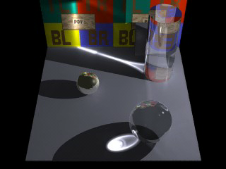
|
|
Reflective caustics |
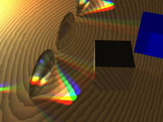
|
Here we have three lenses and three light sources. The middle lens has photon mapping turned off. You can also see some reflective caustics from the brass box (some light reflects and hits the blue box, other light bounces through the nearest lens and is focused in the lower left corner of the image). |
|
Photons used for lenses and caustics |
3.4.4.4.2 Using Photon Mapping in Your Scene
When designing a scene with photons, it helps to think of the scene objects in two categories. Objects in the first category will show photon caustics when hit by photons. Objects in the second category cause photon caustics by reflecting or refracting photons. Some objects may be in both categories, and some objects may be in neither category.
Category 1 - Objects that show photon caustics
By default, all objects are in the first category. Whenever a photon hits
an object, the photon is stored and will later be used to render caustics on
that object. This means that, by default, caustics from photons can appear
on any surface. To speed up rendering, you can take objects out of this
category. You do this with the line: photons{collect off}. If you use
this syntax, caustics from photons will not appear on the object. This will
save both memory and computational time during rendering.
Category 2 - Objects that cause photon caustics
By default, there are no objects in the second category. If you want your
object to cause caustics, you need to do two things. First, make your object into
a "target." You do this with the target keyword. This enables light
sources to shoot photons at your object. Second, you need to specify if
your object reflects photons, refracts photons, or both. This is done with
the reflection on and refraction on keywords. To allow an object to
reflect and refract photons, you would use the following lines of code
inside the object:
photons{
  target
  reflection on
  refraction on
  }
Generally speaking, you do not want an object to be in both categories. Most objects that cause photon caustics do not themselves have much color or brightness. Usually they simply refract or reflect their surroundings. For this reason, it is usually a waste of time to display photon caustics on such surfaces. Even if computed, the effects from the caustics would be so dim that they would go unnoticed.
Sometimes, you may also wish to add photons{collect off} to other clear or
reflective objects, even if they are not photon targets. Again, this is
done to prevent unnecessary computation of caustic lighting.
Finally, you may wish to enable photon reflection and refraction for a surface, even if it is not a target. This allows indirect photons (photons that have already hit a target and been reflected or refracted) to continue their journey after hitting this object.
3.4.4.4.3 Photon Global Settings
global_photon_block:

photons {
  spacing <photon_spacing> | count <photons_to_shoot>
  [gather <min_gather>, <max_gather>]
  [media <max_steps> [,<factor>]]
  [jitter <jitter_amount>]
  [max_trace_level <photon_trace_level>]
  [adc_bailout <photon_adc_bailout>]
  [save_file "filename" | load_file "filename"]
  [autostop <autostop_fraction>]
  [expand_thresholds <percent_increase>, <expand_min>]
  [radius <gather_radius>, <multiplier>, <gather_radius_media>,<multiplier>]
  }
All photons default values:
Global :
expand_min    : 40
gather        : 20, 100
jitter        : 0.4
media         : 0

Object :
collect       : on
refraction    : off
reflection    : off
split_union   : on
target        : 1.0

Light_source:
area_light    : off
refraction    : off
reflection    : off
To specify photon gathering and storage options you need to add a photons
block to the global_settings section of your scene.
For example:
global_settings {
  photons {
    count 20000
    autostop 0
    jitter .4
    }
  }
The number of photons generated can be set using either the spacing or count keywords:
- If spacing is used, it specifies approximately the average distance between photons on surfaces. If you cut the spacing in half, you will get four times as many surface photons, and eight times as many media photons.
- If count is used, POV-Ray will shoot the approximately number of photons
specified. The actual number of photons that result from this will almost
always be at least slightly different from the number specified. Still, if you
double the photons_to_shoot value, then twice as many photons will be shot. If
you cut the value in half, then half the number of photons will be shot.
- It may be less, because POV shoots photons at a target object's bounding box, which means that some photons will miss the target object.
- On the other hand, may be more, because each time one object hits an object that has both reflection and refraction, two photons are created (one for reflection and one for refraction).
- POV will attempt to compensate for these two factors, but it can only estimate how many photons will actually be generated. Sometimes this estimation is rather poor, but the feature is still usable.
The keyword gather allows you to specify how many photons are
gathered at each point during the regular rendering step. The first number
(default 20) is the minimum number to gather, while the second number (default
100) is the maximum number to gather. These are good values and you should only
use different ones if you know what you are doing.
The keyword media turns on media photons. The parameter
max_steps specifies the maximum number of photons to deposit
over an interval. The optional parameter factor specifies the difference in
media spacing compared to surface spacing. You can increase factor and
decrease max_steps if too many photons are being deposited in media.
The keyword jitter specifies the amount of jitter used in the
sampling of light rays in the pre-processing step. The default value is good and
usually does not need to be changed.
The keywords max_trace_level and adc_bailout allow
you to specify these attributes for the photon-tracing step. If you do not
specify these, the values for the primary ray-tracing step will be used.
The keywords save_file and load_file allow you to
save and load photon maps. If you load a photon map, no photons will be shot.
The photon map file contains all surface (caustic) and media
photons.
radius is used for gathering photons. The larger the radius, the longer it
takes to gather photons. But if you use too small of a radius, you might
not get enough photons to get a good estimate. Therefore, choosing a good
radius is important. Normally POV-Ray looks through the photon map and uses some ad-hoc statistical analysis to determine a reasonable radius. Sometimes it does a good job, sometimes it does not. The radius keyword lets you override or adjust POV-Ray's guess.
radius parameters (all are optional):
- Manually set the gather radius for surface photons. If this is either zero or if you leave it out, POV-Ray will analyze and guess.
- Adjust the radius for surface photons by setting a multiplier. If POV-Ray, for example, is picking a radius that you think is too big (render is too slow), you can use
radius ,0.5to lower the radius (multiply by 0.5) and speed up the render at the cost of quality. - Manually set the gather radius for media photons.
- Adjust the radius for media photons by setting a multiplier.
The keywords autostop
and expand_thresholds will be explained later.
3.4.4.4.4 Shooting Photons at an Object
object_photon_block:
photons {
  [target [Float]]
  [refraction on|off]
  [reflection on|off]
  [collect on|off]
  [pass_through]
  }
To shoot photons at an object, you need to tell POV that the object receives
photons. To do this, create a photons { } block within the object. For example:
object {
  MyObject
  photons {
    target
    refraction on
    reflection on
    collect off
    }
  }
In this example, the object both reflects and refracts photons. Either of these options could be turned off (by specifying reflection off, for example). By using this, you can have an object with a reflective finish which does not reflect photons for speed and memory reasons.
The keyword target makes this object a target.
The density of the photons can be adjusted by specifying a spacing multiplier in the form of an optional value after the target keyword. If, for example, you specify a spacing multiplier of 0.5, then the spacing for photons hitting this object will be 1/2 of the distance of the spacing for other objects.
Note: This means four times as many surface photons, and eight times as many media photons.
The keyword collect off causes the object to ignore photons.
Photons are neither deposited nor gathered on that object.
The keyword pass_through causes photons to pass through the
object unaffected on their way to a target object. Once a
photon hits the target object, it will ignore the pass_through
flag. This is basically a photon version of the no_shadow
keyword, with the exception that media within the object will still be
affected by the photons (unless that media specifies collect off). If you
use the no_shadow keyword, the object will be tagged as
pass_through automatically. You can then turn off
pass_through if necessary by simply using photons {
pass_through off }.
Note: Photons will not be shot at an object unless you
specify the target keyword. Simply turning refraction on will not
suffice.
When shooting photons at a CSG-union, it may sometimes be of advantage to use
split_union off inside the union.
POV-Ray will be forced to shoot at the whole object, instead of splitting it up
and shooting photons at its compound parts.
3.4.4.4.5 Photons and Light Sources
light_photon_block:
photons {
  [refraction on | off]
  [reflection on | off]
  [area_light]
  }
Example:
light_source {
  MyLight
  photons {
    refraction on
    reflection on
    }
  }
Sometimes, you want photons to be shot from one light source and not another. In that case, you can turn photons on for an object, but specify photons {reflection off refraction off } in the light source's definition. You can also turn off only reflection or only refraction for any light source.
Note: The photon shooting performance has been improved with the addition of multiple-thread support. To take advantage of this at the moment, your scene will need multiple light sources.
3.4.4.4.6 Photons and Media
global_settings {
  photons {
    count 10000
    media 100
    }
  }
Photons also interact fully with media. This means that volumetric photons are stored in scattering media. This is enabled by using the keyword media within the photons block.
To store photons in media, POV deposits photons as it steps through the media during the photon-tracing phase of the render. It will deposit these photons as it traces caustic photons, so the number of media photons is dependent on the number of caustic photons. As a light ray passes through a section of media, the photons are deposited, separated by approximately the same distance that separates surface photons.
You can specify a factor as a second optional parameter to the media keyword. If, for example, factor is set to 2.0, then photons will be spaced twice as far apart as they would otherwise have been spaced.
Sometimes, however, if a section of media is very large, using these settings could create a large number of photons very fast and overload memory. Therefore, following the media keyword, you must specify the maximum number of photons that are deposited for each ray that travels through each section of media. A setting of 100 should probably work in most cases.
You can put collect off into media to make that media ignore
photons. Photons will neither be deposited nor gathered in a media that is
ignoring them. Photons will also not be gathered nor deposited in non-scattering
media. However, if multiple medias exist in the same space, and at least
one does not ignore photons and is scattering, then photons will be deposited in
that interval and will be gathered for use with all media in that interval.
3.4.4.4.7 Photons FAQ
I made an object with IOR 1.0 and the shadows look weird.
If the borders of your shadows look odd when using photon mapping, do not be alarmed. This is an unfortunate side-effect of the method. If you increase the density of photons (by decreasing spacing and gather radius) you will notice the problem diminish. We suggest not using photons if your object does not cause much refraction (such as with a window pane or other flat piece of glass or any objects with an IOR very close to 1.0).
My scene takes forever to render.
When POV-Ray builds the photon maps, it continually displays in the status bar the number of photons that have been shot. Is POV-Ray stuck in this step and does it keep shooting lots and lots of photons?
yes
If you are shooting photons at an infinite object (like a plane), then you should expect this. Either be patient or do not shoot photons at infinite objects.
Are you shooting photons at a CSG difference? Sometimes POV-Ray does a bad
job creating bounding boxes for these objects. And since photons are shot at the
bounding box, you could get bad results. Try manually bounding the object. You
can also try the autostop feature (try autostop 0). See the docs
for more info on autostop.
no
Does your scene have lots of glass (or other clear objects)? Glass is slow and you need to be patient.
My scene has polka dots but renders really quickly. Why?
You should increase the number of photons (or decrease the spacing).
The photons in my scene show up only as small, bright dots. How can I fix this?
The automatic calculation of the gather radius is probably not working correctly, most likely because there are many photons not visible in your scene which are affecting the statistical analysis.
You can fix this by either reducing the number of photons that are in your scene but not visible to the camera (which confuse the auto-computation), or by specifying the initial gather radius manually by using the keyword radius. If you must manually specify a gather radius, it is usually best to also use spacing instead of count, and then set radius and spacing to a 5:1 (radius:spacing) ratio.
Adding photons slowed down my scene a lot, and I see polka dots.
This is usually caused by having both high- and low-density photons in the same scene. The low density ones cause polka dots, while the high density ones slow down the scene. It is usually best if the all photons are on the same order of magnitude for spacing and brightness. Be careful if you are shooting photons objects close to and far from a light source. There is an optional parameter to the target keyword which allows you to adjust the spacing of photons at the target object. You may need to adjust this factor for objects very close to or surrounding the light source.
I added photons, but I do not see any caustics.
When POV-Ray builds the photon maps, it continually displays in the status bar the number of photons that have been shot. Did it show any photons being shot?
no
Try avoiding autostop, or you might want to bound your object
manually.
Try increasing the number of photons (or decreasing the spacing).
yes
Were any photons stored (the number after total in the
rendering message as POV-Ray shoots photons)?
no
It is possible that the photons are not hitting the target object (because another object is between the light source and the other object).
yes
The photons may be diverging more than you expect. They are probably there, but you cannot see them since they are spread out too much
The base of my glass object is really bright.
Use collect off with that object.
Will area lights work with photon mapping?
Photons do work with area lights. However, normally photon mapping ignores
all area light options and treats all light sources as point lights. If you
would like photon mapping to use your area light options, you must specify the
"area_light" keyword within the photons {
} block in your light source's code. Doing this will not increase the
number of photons shot by the light source, but it might cause regular patterns
to show up in the rendered caustics (possibly splotchy).
What do the stats mean?
In the stats, photons shot means how many light rays were shot
from the light sources. photons stored means how many photons are
deposited on surfaces in the scene. If you turn on reflection and refraction,
you could get more photons stored than photons shot, since the each ray can get
split into two.
3.4.4.4.8 Photon Tips
- Use
collect offin objects that photons do not hit. Just putphotons { collect off }in the object's definition. - Use
collect offin glass objects. - Use
autostopunless it causes problems. - A big tip is to make sure that all of the final densities of photons are of the same general magnitude. You do not want spots with really high density photons and another area with really low density photons. You will always have some variation (which is a good thing), but having really big differences in photon density is what causes some scenes to take many hours to render.
3.4.4.4.9 Advanced Techniques
3.4.4.4.9.1 Autostop
|
To understand the |
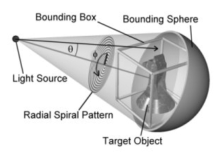
|
|
Example of the photon autostop option |
Normally, POV does not stop shooting photons until the target object's
entire bounding box has been thoroughly covered. Sometimes, however, an object
is much smaller than its bounding box. At these times, we want to stop shooting
if we do a complete circle in the spiral without hitting the object.
Unfortunately, some objects (such as copper rings), have holes in the middle.
Since we start shooting at the middle of the object, the photons just go through
the hole in the middle, thus fooling the system into thinking that
it is done. To avoid this, the autostop keyword lets you specify
how far the system must go before this auto-stopping feature kicks in. The value
specified is a fraction of the object's bounding box. Valid values are 0.0
through 1.0 (0% through 100%). POV will continue to shoot photons until the
spiral has exceeded this value or the bounding box is completely covered. If a
complete circle of photons fails to hit the target object after the spiral has
passed the autostop threshold, POV will then stop shooting photons.
The autostop feature will also not kick in until at least one
photon has hit the object. This allows you to use autostop 0 even
with objects that have holes in the middle.
Note: If the light source is within the object's bounding box, the photons are shot in all directions from the light source.
3.4.4.4.9.2 Adaptive Search Radius
Unless photons are interacting with media, POV-Ray uses an adaptive search radius while gathering photons. If the minimum number of photons is not found in the original search radius, the radius is expanded and searched again. Using this adaptive search radius can both decrease the amount of time it takes to render the image, and sharpen the borders in the caustic patterns.
Sometimes this adaptive search technique can create unwanted artifacts at
borders. To remove these artifacts, a few thresholds are used, which can be
specified by expand_thresholds. For example, if expanding the
radius increases the estimated density of photons by too much (threshold is
percent_increase, default is 20%, or 0.2), the expanded search is discarded and
the old search is used instead. However, if too few photons are gathered in the
expanded search (expand_min, default is 40), the new search will be
used always, even if it means more than a 20% increase in photon density.
3.4.4.4.9.3 Photons and Dispersion
When dispersion is specified for interior of a transparent object, photons will make use of that and show "colored" caustics.
3.4.4.4.9.4 Saving and Loading Photon Maps
It is possible to save and load photon maps to speed up rendering. The photon map itself is view-independent, so if you want to animate a scene that contains photons and you know the photon map will not change during the animation, you can save it on the first frame and then load it for all subsequent frames.
To save the photon map, put the line
save_file "myfile.ph"
into the photons { } block inside the global_settings section.
Loading the photon map is the same, but with load_file instead
of save_file. You cannot both load and save a photon map in the POV
file. If you load the photon map, it will load all of the photons. No photons will be shot if the map is loaded
from a file. All other options (such as gather radius) must still be specified
in the POV scene file and are not loaded with the photon map.
When can you safely re-use a saved photon map?
- Moving the camera is always safe.
- Moving lights that do not cast photons is always safe.
- Moving objects that do not have photons shot at them, that do not receive photons, and would not receive photons in the new location is always safe.
- Moving an object that receives photons to a new location where it does not receive photons is sometimes safe.
- Moving an object to a location where it receives photons is not safe
- Moving an object that has photons shot at it is not safe
- Moving a light that casts photons is not safe.
- Changing the texture of an object that receives photons is safe.
- Changing the texture of an object that has photons shot at it produces results that are not realistic, but can be useful sometimes.
In general, changes to the scene geometry require photons to be re-shot. Changing the camera parameters or changing the image resolution does not.
3.4.5 Object
Objects are the building blocks of your scene. There are a lot of different types of objects supported by POV-Ray. In the following sections, we describe Finite Solid Primitives, Finite Patch Primitives and Infinite Solid Primitives. These primitive shapes may be combined into complex shapes using Constructive Solid Geometry (also known as CSG).
The basic syntax of an object is a keyword describing its type, some floats, vectors or other parameters which further define its location and/or shape and some optional object modifiers such as texture, interior_texture, pigment, normal, finish, interior, bounding, clipping or transformations. Specifically the syntax is:
OBJECT:
  FINITE_SOLID_OBJECT | FINITE_PATCH_OBJECT |
  INFINITE_SOLID_OBJECT | CSG_OBJECT | LIGHT_SOURCE |
  object { OBJECT_IDENTIFIER [OBJECT_MODIFIERS...] }
FINITE_SOLID_OBJECT:
  BLOB | BOX | CONE | CYLINDER | HEIGHT_FIELD | ISOSURFACE | JULIA_FRACTAL |
  LATHE | OVUS | PARAMETRIC | PRISM | SPHERE | SPHERE_SWEEP | SUPERELLIPSOID |
  SOR | TEXT | TORUS
FINITE_PATCH_OBJECT:
  BICUBIC_PATCH | DISC | MESH | MESH2 | POLYGON | TRIANGLE |
  SMOOTH_TRIANGLE
  INFINITE_SOLID_OBJECT:
  PLANE | POLY | CUBIC | QUARTIC | QUADRIC
CSG_OBJECT:
  UNION | INTERSECTION | DIFFERENCE | MERGE
Object identifiers may be declared to make scene files more readable and to parameterize scenes so that changing a single declaration changes many values. An identifier is declared as follows.
OBJECT_DECLARATION:
  #declare IDENTIFIER = OBJECT |
  #local IDENTIFIER = OBJECT
Where IDENTIFIER is the name of the identifier up to 40
characters long and OBJECT is any valid object. To invoke
an object identifier, you wrap it in an object{...} statement.
You use the object statement regardless of what type of object
it originally was. Although early versions of POV-Ray required this
object wrapper all of the time, now it is only used with
OBJECT_IDENTIFIERS.
Object modifiers are covered in detail later. However here is a brief overview.
The texture describes the surface properties of the object. Complete details are in textures. Textures are combinations of pigments, normals, and finishes. In the section pigment you will learn how to specify the color or pattern of colors inherent in the material. In normal, we describe a method of simulating various patterns of bumps, dents, ripples or waves by modifying the surface normal vector. The section on finish describes the reflective properties of the surface. The Interior is a feature introduced in POV-Ray 3.1. It contains information about the interior of the object which was formerly contained in the finish and halo parts of a texture. Interior items are no longer part of the texture. Instead, they attach directly to the objects. The halo feature has been discontinued and replaced with a new feature called Media which replaces both halo and atmosphere.
Bounding shapes are finite, invisible shapes which wrap around complex, slow rendering shapes in order to speed up rendering time. Clipping shapes are used to cut away parts of shapes to expose a hollow interior. Transformations tell the ray-tracer how to move, size or rotate the shape and/or the texture in the scene.
3.4.5.1 Finite Solid Primitives
There are seventeen different solid finite primitive shapes: blob, box, cone, cylinder, height field, isosurface, Julia fractal, lathe, ovus, parametric, prism, sphere, sphere_sweep, superellipsoid, surface of revolution, text and torus. These have a well-defined inside and can be used in CSG: see Constructive Solid Geometry. They are finite and respond to automatic bounding. You may specify an interior for these objects.
3.4.5.1.1 Blob
Blobs are an interesting and flexible object type. Mathematically they are iso-surfaces of scalar fields, i.e. their surface is defined by the strength of the field in each point. If this strength is equal to a threshold value you are on the surface otherwise you are not.
Picture each blob component as an object floating in space. This object is filled with a field that has its maximum at the center of the object and drops off to zero at the object's surface. The field strength of all those components are added together to form the field of the blob. Now POV-Ray looks for points where this field has a given value, the threshold value. All these points form the surface of the blob object. Points with a greater field value than the threshold value are considered to be inside while points with a smaller field value are outside.
There's another, simpler way of looking at blobs. They can be seen as a union of flexible components that attract or repel each other to form a blobby organic looking shape. The components' surfaces actually stretch out smoothly and connect as if they were made of honey or something similar.
The syntax for blob is defined as follows:
BLOB:
  blob { BLOB_ITEM... [BLOB_MODIFIERS...]}
BLOB_ITEM:
  sphere{<Center>, Radius,
    [ strength ] Strength[COMPONENT_MODIFIER...] } |
  cylinder{<End1>, <End2>, Radius,
    [ strength ] Strength [COMPONENT_MODIFIER...] } |
  component Strength, Radius, <Center> |
  threshold Amount
COMPONENT_MODIFIER:
  TEXTURE | PIGMENT | NORMAL | FINISH | TRANSFORMATION
BLOB_MODIFIER:
  hierarchy [Boolean] | sturm [Boolean] | OBJECT_MODIFIER
Blob default values:
hierarchy : on
sturm     : off
threshold : 1.0
The threshold keyword is followed by a float value which
determines the total field strength value that POV-Ray is looking for. The
default value if none is specified is threshold 1.0. By
following the ray out into space and looking at how each blob component
affects the ray, POV-Ray will find the points in space where the field
strength is equal to the threshold value. The following list shows some
things you should know about the threshold value.
- The threshold value must be positive.
- A component disappears if the threshold value is greater than its strength.
- As the threshold value gets larger, the surface you see gets closer to the centers of the components.
- As the threshold value gets smaller, the surface you see gets closer to the surface of the components.
Cylindrical components are specified by a cylinder statement.
The center of the end-caps of the cylinder is defined by the vectors
<End1> and <End2>. Next
is the float value of the Radius followed by the float
Strength. These vectors and floats are required and should be separated
by commas. The keyword strength may optionally precede the
strength value. The cylinder has hemispherical caps at each end.
Spherical components are specified by a sphere statement. The
location is defined by the vector <Center>. Next
is the float value of the Radius followed by the float
Strength. These vector and float values are required and should be
separated by commas. The keyword strength may optionally
precede the strength value.
You usually will apply a single texture to the entire blob object, and you
typically use transformations to change its size, location, and orientation.
However both the cylinder and sphere statements may
have individual texture, pigment, normal, finish, and transformations applied
to them. You may not apply separate interior statements to the
components but you may specify one for the entire blob.
Note: By unevenly scaling a spherical component you can create ellipsoidal components. The tutorial section on Blob Object illustrates individually textured blob components and many other blob examples.
The component keyword is an obsolete method for specifying a
spherical component and is only used for compatibility with earlier POV-Ray
versions. It may not have textures or transformations individually applied to
it.
The strength parameter of either type of blob component is a
float value specifying the field strength at the center of the object. The
strength may be positive or negative. A positive value will make that
component attract other components while a negative value will make it repel
other components. Components in different, separate blob shapes do not affect
each other.
You should keep the following things in mind.
- The strength value may be positive or negative. Zero is a bad value, as the net result is that no field was added -- you might just as well have not used this component.
- If strength is positive, then POV-Ray will add the component's field to the space around the center of the component. If this adds enough field strength to be greater than the threshold value you will see a surface.
- If the strength value is negative, then POV-Ray will subtract the component's field from the space around the center of the component. This will only do something if there happen to be positive components nearby. The surface around any nearby positive components will be dented away from the center of the negative component.
After all components and the optional threshold value have
been specified you may specify zero or more blob modifiers. A blob modifier
is any regular object modifier or the hierarchy or
sturm keywords.
The components of each blob object are internally bounded by a spherical
bounding hierarchy to speed up blob intersection tests and other operations.
Using the optional keyword hierarchy followed by an optional
boolean float value will turn it off or on. By default it is on.
The calculations for blobs must be very accurate. If this shape renders
improperly you may add the keyword sturm followed by an
optional boolean float value to turn off or on POV-Ray's
slower-yet-more-accurate Sturmian root solver. By default it is off.
An example of a three component blob is:
BLOB:
  blob {
    threshold 0.6
      sphere { <.75, 0, 0>, 1, 1 }
      sphere { <-.375, .64952, 0>, 1, 1 }
      sphere { <-.375, -.64952, 0>, 1, 1 }
    scale 2
    }
If you have a single blob component then the surface you see will just look like the object used, i.e. a sphere or a cylinder, with the surface being somewhere inside the surface specified for the component. The exact surface location can be determined from the blob equation listed below (you will probably never need to know this, blobs are more for visual appeal than for exact modeling).
For the more mathematically minded, here's the formula used internally by POV-Ray to create blobs. You do not need to understand this to use blobs. The density of the blob field of a single component is:
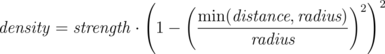
|
|
Blob Density |
where distance is the distance of a given point from the spherical blob's center or cylinder blob's axis. This formula has the nice property that it is exactly equal to the strength parameter at the center of the component and drops off to exactly 0 at a distance from the center of the component that is equal to the radius value. The density formula for more than one blob component is just the sum of the individual component densities.
3.4.5.1.2 Box
A simple box can be defined by listing two corners of the box using the
following syntax for a box statement:
BOX:
  box {
    <Corner_1>, <Corner_2>
    [OBJECT_MODIFIERS...]
    }
|
|
The geometry of a box. |
Where <Corner_1> and
<Corner_2> are vectors defining the x, y, z coordinates of
the opposite corners of the box.
Note: All boxes are defined with their faces parallel to the coordinate axes. They may later be rotated to any orientation using the rotate keyword.
Boxes are calculated efficiently and make good bounding shapes (if manually bounding seems to be necessary).
3.4.5.1.3 Cone
The cone statement creates a finite length cone or a
frustum (a cone with the point cut off). The syntax is:
CONE:
  cone {
    <Base_Point>, Base_Radius, <Cap_Point>, Cap_Radius
    [ open ][OBJECT_MODIFIERS...]
    }
|
|
The geometry of a cone. |
Where <Base_Point> and <
Cap_Point> are vectors defining the x, y, z coordinates of the
center of the cone's base and cap and Base_Radius
and Cap_Radius are float values for the corresponding
radii.
Normally the ends of a cone are closed by flat discs that are parallel to
each other and perpendicular to the length of the cone. Adding the optional
keyword open after Cap_Radius will remove
the end caps and results in a tapered hollow tube like a megaphone or
funnel.
3.4.5.1.4 Cylinder
The cylinder statement creates a finite length cylinder with
parallel end caps The syntax is:
CYLINDER:
  cylinder {
    <Base_Point>, <Cap_Point>, Radius
    [ open ][OBJECT_MODIFIERS...]
    }
|
|
The geometry of a cylinder. |
Where <Base_Point> and
<Cap_Point> are vectors defining the x, y, z coordinates of
the cylinder's base and cap and Radius is a float
value for the radius.
Normally the ends of a cylinder are closed by flat discs that are parallel
to each other and perpendicular to the length of the cylinder. Adding the
optional keyword open after the radius will remove the end caps
and results in a hollow tube.
3.4.5.1.5 Height Field
Height fields are fast, efficient objects that are generally used to
create mountains or other raised surfaces out of hundreds of triangles in a
mesh. The height_field statement syntax is:
HEIGHT_FIELD:
  height_field {
    [HF_TYPE] "filename" [gamma GAMMA] [premultiplied BOOL] | [HF_FUNCTION]
    [HF_MODIFIER...]
    [OBJECT_MODIFIER...]
    }
HF_TYPE:
  exr | gif | hdr | iff | jpeg | pgm | png | pot | ppm | sys | tga | tiff
HF_FUNCTION:
  function FieldResolution_X, FieldResolution_Y { UserDefined_Function }
HF_MODIFIER:
  smooth & water_level Level
OBJECT_MODIFIER:
  hierarchy [Boolean]
Height_field default values:
hierarchy   : on
smooth      : off
water_level : 0.0
A height field is essentially a one unit wide by one unit long square with a mountainous surface on top. The height of the mountain at each point is taken from the color number or palette index of the pixels in a graphic image file. The maximum height is one, which corresponds to the maximum possible color or palette index value in the image file.
|
|
The size and orientation of an unscaled height field. |
The mesh of triangles corresponds directly to the pixels in the image
file. Each square formed by four neighboring pixels is divided into two
triangles. An image with a resolution of N*M pixels has
(N-1)*(M-1) squares that are divided into
2*(N-1)*(M-1) triangles.
|
|
Relationship of pixels and triangles in a height field. |
The resolution of the height field is influenced by two factors: the resolution of the image and the resolution of the color/index values. The size of the image determines the resolution in the x- and z-direction. A larger image uses more triangles and looks smoother. The resolution of the color/index value determines the resolution along the y-axis. A height field made from an 8-bit image can have 256 different height levels while one made from a 16-bit image can have up to 65536 different height levels. Thus the second height field will look much smoother in the y-direction if the height field is created appropriately.
The size/resolution of the image does not affect the size of the height field. The unscaled height field size will always be 1 by 1 by 1. Higher resolution image files will create smaller triangles, not larger height fields.
The image file type used to create a height field is specified by one of the keywords listed above. Specifying the file type is optional. If it is not defined the same file type will be assumed as the one that is set as the output file type. This is useful when the source for the height_field is also generated with POV-Ray.
The GIF, PNG, PGM, TIFF and possibly SYS format files are the only ones that can be created using a standard paint program. Though there are paint programs for creating TGA image files they will not be of much use for creating the special 16 bit TGA files used by POV-Ray (see below and HF_Gray_16 for more details).
In an image file that uses a color palette, like GIF, the color number is the palette index at a given pixel. Use a paint program to look at the palette of a GIF image. The first color is palette index zero, the second is index one, the third is index two and so on. The last palette entry is index 255. Portions of the image that use low palette entries will result in lower parts of the height field. Portions of the image that use higher palette entries will result in higher parts of the height field.
Height fields created from GIF files can only have 256 different height levels because the maximum number of colors in a GIF file is 256.
The color of the palette entry does not affect the height of the pixel. Color entry 0 could be red, blue, black or orange but the height of any pixel that uses color entry 0 will always be 0. Color entry 255 could be indigo, hot pink, white or sky blue but the height of any pixel that uses color entry 255 will always be 1.
You can create height field GIF images with a paint program or a fractal program like Fractint.
A POT file is essentially a GIF file with a 16 bit palette. The maximum number of colors in a POT file is 65536. This means a POT height field can have up to 65536 possible height values. This makes it possible to have much smoother height fields.
Note: The maximum height of the field is still 1 even though more intermediate values are possible.
At the time of this writing the only program that created POT files was a freeware MS-Dos/Windows program called Fractint. POT files generated with this fractal program create fantastic landscapes.
The TGA and PPM file formats may be used as a storage device for 16 bit numbers rather than an image file. These formats use the red and green bytes of each pixel to store the high and low bytes of a height value. These files are as smooth as POT files but they must be generated with special custom-made programs. Several programs can create TGA heightfields in the format POV uses, such as Gforge and Terrain Maker.
PNG format heightfields are usually stored in the form of a grayscale image with black corresponding to lower and white to higher parts of the height field. Because PNG files can store up to 16 bits in grayscale images they will be as smooth as TGA and PPM images. Since they are grayscale images you will be able to view them with a regular image viewer. Gforge can create 16-bit heightfields in PNG format. Color PNG images will be used in the same way as TGA and PPM images.
SYS format is a platform specific file format. See your platform specific documentation for details.
In addition to all the usual object modifiers, there are three additional height field modifiers available.
The optional water_level parameter may be added after the file
name. It consists of the keyword water_level followed by a
float value telling the program to ignore parts of the height field below
that value. The default value is zero and legal values are between zero and
one. For example water_level 0.5 tells POV-Ray to only render
the top half of the height field. The other half is below the water
and could not be seen anyway. Using water_level renders
faster than cutting off the lower part using CSG or clipping. This term comes
from the popular use of height fields to render landscapes. A height field
would be used to create islands and another shape would be used to simulate
water around the islands. A large portion of the height field would be
obscured by the water so the water_level parameter was
introduced to allow the ray-tracer to ignore the unseen parts of the height
field. water_level is also used to cut away unwanted lower
values in a height field. For example if you have an image of a fractal on a
solid colored background, where the background color is palette entry 0, you
can remove the background in the height field by specifying,
water_level 0.001.
Normally height fields have a rough, jagged look because they are made of
lots of flat triangles. Adding the keyword smooth causes
POV-Ray to modify the surface normal vectors of the triangles in such a way
that the lighting and shading of the triangles will give a smooth look. This
may allow you to use a lower resolution file for your height field than would
otherwise be needed. However, smooth triangles will take longer to render.
The default value is off.
In order to speed up the intersection tests a one-level bounding hierarchy
is available. By default it is always used but it can be switched off using
hierarchy off to improve the rendering speed for small height
fields (i.e. low resolution images). You may optionally use a boolean value
such as hierarchy on or hierarchy off.
While POV-Ray will normally interpret the height field input file as a container of linear data irregardless of file type, this can be overridden for any individual height field input file by specifying gamma GAMMA immediately after the file name. For example:
height field {
  jpeg "foobar.jpg" gamma 1.8
  }
This will cause POV-Ray to perform gamma adjustment or -decoding on the input file data before building the height field. Alternatively to a numerical value, srgb may be specified to denote that the file format is pre-corrected or encoded using the ''sRGB transfer function'' instead of a power-law gamma function. See the section Gamma Handling for more information.
The height field object also allows for substituting a user defined function instead of specifying an image. That function can either be in it's literal form, or it can be a call to a function that you have predeclared. The user supplied parameters FieldResolution_X and FieldResolution_Y are integer values that affect the resolution of the color/index values, not size of the unscaled height field.
3.4.5.1.6 Isosurface
Details about many of the things that can be done with the isosurface object are discussed in the isosurface tutorial section. Below you will only find the syntax basics:
isosurface {
  function { FUNCTION_ITEMS }
  [contained_by { SPHERE | BOX }]
  [threshold FLOAT_VALUE]
  [accuracy FLOAT_VALUE]
  [max_gradient FLOAT_VALUE]
  [evaluate P0, P1, P2]
  [open]
  [max_trace INTEGER] | [all_intersections]
  [OBJECT_MODIFIERS...]
  }
Isosurface default values:
contained_by : box{-1,1}
threshold    : 0.0
accuracy     : 0.001
max_gradient : 1.1
function { ... } This must be specified and be the first item of the
isosurface statement. Here you place all the mathematical functions that
will describe the surface.
contained_by { ... } The contained_by object limits the
area where POV-Ray samples for the surface of the function. This container can either be a
sphere or a box, both of which use the standard POV-Ray syntax. If not specified a
box {<-1,-1,-1>, <1,1,1>} will be used as default.
contained_by { sphere { CENTER, RADIUS } }
contained_by { box { CORNER1, CORNER2 } }
threshold This specifies how much strength, or substance to give the
isosurface. The surface appears where the function value
equals the threshold value. The default threshold is 0.
function = threshold
accuracy The isosurface finding method is a recursive subdivision method.
This subdivision goes on until the length of the interval where POV-Ray finds a surface
point is less than the specified accuracy. The default value is 0.001.
Smaller values produces more accurate surfaces, but it takes longer to render.
max_gradient POV-Ray can find the first intersecting point between a ray and
the isosurface of any continuous function if the maximum gradient of the function
is known. Therefore you can specify a max_gradient for the function.
The default value is 1.1. When the max_gradient used to find the
intersecting point is too high, the render slows down considerably. When it is too
low, artifacts or holes may appear on the isosurface. When it is way too low, the surface
does not show at all. While rendering the isosurface POV-Ray records the found gradient values
and prints a warning if these values are higher or much lower than the specified
max_gradient:
Warning: The maximum gradient found was 5.257, but max_gradient of
the isosurface was set to 5.000. The isosurface may contain holes!
Adjust max_gradient to get a proper rendering of the isosurface.
Warning: The maximum gradient found was 5.257, but max_gradient of
the isosurface was set to 7.000. Adjust max_gradient to
get a faster rendering of the isosurface.
For best performance you should specify a value close to the real maximum gradient.
evaluate POV-Ray can also dynamically adapt the used max_gradient.
To activate this technique you have to specify the evaluate keyword
followed by three parameters:
- P0: the minimum max_gradient in the estimation process,
- P1: an over-estimating factor. This means that the max_gradient is multiplied by the P1 parameter.
- P2: an attenuation parameter (1 or less)
In this case POV-Ray starts with the max_gradient value P0
and dynamically changes it during the render using P1 and P2.
In the evaluation process, the P1 and P2 parameters are used in
quadratic functions. This means that over-estimation increases more
rapidly with higher values and attenuation more rapidly with lower
values. Also with dynamic max_gradient, there can be artifacts and holes.
If you are unsure what values to use, start a render without evaluate to get
a value for max_gradient. Now you can use it with evaluate like this:
- P0 : found max_gradient * min_factor
min_factor being a float between 0 and 1 to reduce themax_gradientto a minimum max_gradient. The ideal value for P0 would be the average of the found max_gradients, but we do not have access to that information.
A good starting point is 0.6 for the min_factor - P1 : sqrt(found max_gradient/(found max_gradient * min_factor))
min_factor being the same as used in P0 this will give an over-estimation factor of more than 1, based on your minimum max_gradient and the found max_gradient. - P2 : 1 or less
0.7 is a good starting point.
When there are artifacts / holes in the isosurface, increase the min_factor and / or P2 a bit. Example: when the first run gives a found max_gradient of 356, start with
#declare Min_factor= 0.6;
isosurface {
  ...
  evaluate 356*Min_factor,  sqrt(356/(356*Min_factor)),  0.7
  //evaluate 213.6, 1.29, 0.7
  ...
  }
This method is only an approximation of what happens internally, but it gives faster rendering speeds with the majority of isosurfaces.
open When the isosurface is not fully contained within the contained_by object,
there will be a cross section. Where this happens, you will see the surface of the container.
With the open keyword, these cross section surfaces are removed. The inside of the isosurface
becomes visible.
Note: Using open slows down the render speed, and it is not recommended to use it with CSG operations.
max_trace Isosurfaces can be used in CSG shapes since they are solid finite objects
- if not finite by themselves, they are through the cross section with the container.
By default POV-Ray searches only for the first surface which the ray intersects. But when using an
isosurface in CSG operations, the other surfaces must also be found. Therefore,
the keyword max_trace must be added to the isosurface statement.
It must be followed by an integer value. To check for all surfaces, use the keyword all_intersections instead.
With all_intersections POV-Ray keeps looking until all surfaces are found.
With a max_trace it only checks until that number is reached.
3.4.5.1.7 Julia Fractal
A julia fractal object is a 3-D slice of a 4-D object
created by generalizing the process used to create the classic Julia sets.
You can make a wide variety of strange objects using the
julia_fractal statement including some that look like bizarre blobs of
twisted taffy. The julia_fractal syntax is:
JULIA_FRACTAL:
  julia_fractal {
    <4D_Julia_Parameter>
    [JF_ITEM...] [OBJECT_MODIFIER...]
    }
JF_ITEM:
  ALGEBRA_TYPE | FUNCTION_TYPE | max_iteration Count |
  precision Amt | slice <4D_Normal>, Distance
ALGEBRA_TYPE:
  quaternion | hypercomplex
FUNCTION_TYPE:
  QUATERNATION:
    sqr | cube
  HYPERCOMPLEX:
    sqr | cube | exp | reciprocal | sin | asin | sinh |
    asinh | cos | acos | cosh | acosh | tan | atan |tanh |
    atanh | ln | pwr( X_Val, Y_Val )
Julia Fractal default values:
ALGEBRA_TYPE    : quaternion
FUNCTION_TYPE   : sqr
max_iteration   : 20
precision       : 20
slice, DISTANCE : <0,0,0,1>, 0.0
The required 4-D vector <4D_Julia_Parameter>
is the classic Julia parameter p in the iterated
formula f(h) + p. The julia fractal object is
calculated by using an algorithm that determines whether an arbitrary point
h(0) in 4-D space is inside or outside the object. The
algorithm requires generating the sequence of vectors h(0), h(1),
... by iterating the formula h(n+1) = f(h(n)) + p (n =
0, 1, ..., max_iteration-1) where p is the
fixed 4-D vector parameter of the julia fractal and f()
is one of the functions sqr, cube, ... specified
by the presence of the corresponding keyword. The point
h(0) that begins the sequence is considered inside the julia
fractal object if none of the vectors in the sequence escapes a hypersphere
of radius 4 about the origin before the iteration number reaches the integer
max_iteration value. As you increase max_iteration,
some points escape that did not previously escape, forming the julia fractal.
Depending on the <4D_Julia_Parameter>, the julia
fractal object is not necessarily connected; it may be scattered fractal
dust. Using a low max_iteration can fuse together the dust to
make a solid object. A high max_iteration is more accurate but
slows rendering. Even though it is not accurate, the solid shapes you get
with a low max_iteration value can be quite interesting. If
none is specified, the default is max_iteration 20.
Since the mathematical object described by this algorithm is four-dimensional
and POV-Ray renders three dimensional objects, there must be a way to reduce
the number of dimensions of the object from four dimensions to three. This is
accomplished by intersecting the 4-D fractal with a 3-D plane defined by the slice modifier and then projecting the
intersection to 3-D space. The keyword is followed by 4-D vector and a float
separated by a comma. The slice plane is the 3-D space that is perpendicular
to <4D_Normal> and is
Distance units from the origin. Zero length
<4D_Normal> vectors or a
<4D_Normal> vector with a zero fourth component are
illegal. If none is specified, the default is slice
<0,0,0,1>,0.
You can get a good feel for the four dimensional nature of a julia fractal by
using POV-Ray's animation feature to vary a slice's
Distance parameter. You can make the julia fractal appear from
nothing, grow, then shrink to nothing as
Distance changes, much as the cross section of a 3-D object
changes as it passes through a plane.
The precision parameter is a tolerance used in the
determination of whether points are inside or outside the fractal object.
Larger values give more accurate results but slower rendering. Use as low a
value as you can without visibly degrading the fractal object's
appearance but note values less than 1.0 are clipped at 1.0. The default if
none is specified is precision 20.
The presence of the keywords quaternion or
hypercomplex determine which 4-D algebra is used to calculate the
fractal. The default is quaternion. Both are 4-D generalizations
of the complex numbers but neither satisfies all the field properties (all
the properties of real and complex numbers that many of us slept through in
high school). Quaternions have non-commutative multiplication and
hypercomplex numbers can fail to have a multiplicative inverse for some
non-zero elements (it has been proved that you cannot successfully generalize
complex numbers to four dimensions with all the field properties intact, so
something has to break). Both of these algebras were discovered in the 19th
century. Of the two, the quaternions are much better known, but one can argue
that hypercomplex numbers are more useful for our purposes, since complex
valued functions such as sin, cos, etc. can be generalized to work for
hypercomplex numbers in a uniform way.
For the mathematically curious, the algebraic properties of these two algebras can be derived from the multiplication properties of the unit basis vectors 1 = <1,0,0,0>, i=< 0,1,0,0>, j=<0,0,1,0> and k=< 0,0,0,1>. In both algebras 1 x = x 1 = x for any x (1 is the multiplicative identity). The basis vectors 1 and i behave exactly like the familiar complex numbers 1 and i in both algebras.
ij = k |
jk = i |
ki = j |
ji = -k |
kj = -i |
ik = -j |
ii = jj = kk = -1 |
ijk = -1 |
ij = k |
jk = -i |
ki = -j |
ji = k |
kj = -i |
ik = -j |
ii = jj = kk = -1 |
ijk = 1 |
A distance estimation calculation is used with the quaternion calculations to speed them up. The proof that this distance estimation formula works does not generalize from two to four dimensions but the formula seems to work well anyway, the absence of proof notwithstanding!
The presence of one of the function keywords sqr,
cube, etc. determines which function is used for
f(h) in the iteration formula h(n+1) = f(h(n)) +
p. The default is sqr. Most of the function keywords
work only if the hypercomplex keyword is present. Only
sqr and cube work with quaternion. The
functions are all familiar complex functions generalized to four dimensions.
Function Keyword Maps 4-D value h to:
sqr |
h*h |
cube |
h*h*h |
exp |
e raised to the power h |
reciprocal |
1/h |
sin |
sine of h |
asin |
arcsine of h |
sinh |
hyperbolic sine of h |
asinh |
inverse hyperbolic sine of h |
cos |
cosine of h |
acos |
arccosine of h |
cosh |
hyperbolic cos of h |
acosh |
inverse hyperbolic cosine of h |
tan |
tangent of h |
atan |
arctangent of h |
tanh |
hyperbolic tangent of h |
atanh |
inverse hyperbolic tangent of h |
ln |
natural logarithm of h |
pwr(x,y) |
h raised to the complex power x+iy |
A simple example of a julia fractal object is:
julia_fractal {
  <-0.083,0.0,-0.83,-0.025>
  quaternion
  sqr
  max_iteration 8
  precision 15
  }
The first renderings of julia fractals using quaternions were done by Alan Norton and later by John Hart in the '80's. This POV-Ray implementation follows Fractint in pushing beyond what is known in the literature by using hypercomplex numbers and by generalizing the iterating formula to use a variety of transcendental functions instead of just the classic Mandelbrot z2 + c formula. With an extra two dimensions and eighteen functions to work with, intrepid explorers should be able to locate some new fractal beasts in hyperspace, so have at it!
3.4.5.1.8 Lathe
The lathe is an object generated from rotating a
two-dimensional curve about an axis. This curve is defined by a set of points
which are connected by linear, quadratic, cubic or bezier spline curves. The
syntax is:
LATHE:
  lathe {
    [SPLINE_TYPE] Number_Of_Points, <Point_1>
    <Point_2>... <Point_n>
    [LATHE_MODIFIER...]
    }
SPLINE_TYPE:
  linear_spline | quadratic_spline | cubic_spline | bezier_spline
LATHE_MODIFIER:
  sturm | OBJECT_MODIFIER
Lathe default values:
SPLINE_TYPE   : linear_spline
sturm         : off
The first item is a keyword specifying the type of spline. The default if
none is specified is linear_spline. The required integer value
Number_Of_Points specifies how many two-dimensional
points are used to define the curve. The points follow and are specified by
2-D vectors. The curve is not automatically closed, i.e. the first and last
points are not automatically connected. You will have to do this yourself
if you want a closed curve. The curve thus defined is rotated about the
y-axis to form the lathe object, centered at the origin.
The following examples creates a simple lathe object that looks like a thick cylinder, i.e. a cylinder with a thick wall:
lathe {
  linear_spline
  5,
  <2, 0>, <3, 0>, <3, 5>, <2, 5>, <2, 0>
  pigment {Red}
  }
The cylinder has an inner radius of 2 and an outer radius of 3, giving a wall width of 1. It's height is 5 and it's located at the origin pointing up, i.e. the rotation axis is the y-axis.
Note: The first and last point are equal to get a closed curve.
The splines that are used by the lathe and prism objects are a little bit
difficult to understand. The basic concept of splines is to draw a curve
through a given set of points in a determined way. The default
linear_spline is the simplest spline because it's nothing more
than connecting consecutive points with a line. This means the curve
that is drawn between two points only depends on those two points. No
additional information is taken into account. The other splines are different
in that they do take other points into account when connecting two points.
This creates a smooth curve and, in the case of the cubic spline, produces
smoother transitions at each point.
The quadratic_spline keyword creates splines that are made of
quadratic curves. Each of them connects two consecutive points. Since those
two points (call them second and third point) are not sufficient to describe
a quadratic curve, the predecessor of the second point is taken into account
when the curve is drawn. Mathematically, the relationship (their relative locations on
the 2-D plane) between the first and second point determines the slope of the
curve at the second point. The slope of the curve at the third point is out
of control. Thus quadratic splines look much smoother than linear splines but
the transitions at each point are generally not smooth because the slopes on
both sides of the point are different.
The cubic_spline keyword creates splines which overcome the
transition problem of quadratic splines because they also take a fourth
point into account when drawing the curve between the second and third point.
The slope at the fourth point is under control now and allows a smooth
transition at each point. Thus cubic splines produce the most flexible and
smooth curves.
The bezier_spline is an alternate kind of cubic spline. Points
1 and 4 specify the end points of a segment and points 2 and 3 are control
points which specify the slope at the endpoints. Points 2 and 3 do not
actually lie on the spline. They adjust the slope of the spline. If you draw
an imaginary line between point 1 and 2, it represents the slope at point 1.
It is a line tangent to the curve at point 1. The greater the distance
between 1 and 2, the flatter the curve. With a short tangent the spline can
bend more. The same holds true for control point 3 and endpoint 4. If you
want the spline to be smooth between segments, points 3 and 4 on one segment
and points 1 and 2 on the next segment must form a straight line and point 4
of one segment must be the same as point 1 on the next segment.
You should note that the number of spline segments, i. e. curves between two points, depends on the spline type used. For linear splines you get n-1 segments connecting the points P[i], i=1,...,n. A quadratic spline gives you n-2 segments because the last point is only used for determining the slope, as explained above (thus you will need at least three points to define a quadratic spline). The same holds for cubic splines where you get n-3 segments with the first and last point used only for slope calculations (thus needing at least four points). The bezier spline requires 4 points per segment, creating n/4 segments.
If you want to get a closed quadratic and cubic spline with smooth transitions at the end points you have to make sure that in the cubic case P[n-1] = P[2] (to get a closed curve), P[n] = P[3] and P[n-2] = P[1] (to smooth the transition). In the quadratic case P[n-1] = P[1] (to close the curve) and P[n] = P[2].
The sturm keyword can be used to specify that the slower, but
more accurate, Sturmian root solver should be used. Use it, if the shape does not render properly. Since a quadratic polynomial has to be solved for the linear spline lathe, the Sturmian root solver is not needed.
3.4.5.1.9 Ovus
An ovus is a shape that looks like an egg. The syntax of the ovus object is:
OVUS:
  ovus {
    Bottom_radius, Top_radius
    [OBJECT_MODIFIERS...]
    }
|
Where |
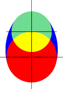 |
|
An ovus 2D section |
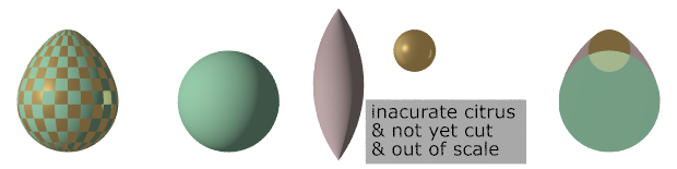 |
The ovus and it's constituent 3D shapes |
Whenever the top radius is bigger than twice the bottom radius, the ovus degenerates into a sphere with an offset center. There are a lot of variations in the shape of the ovus.
Note: According to the ratio of the radius, the pointy part is the smallest radius, but is not always on top!
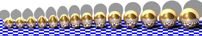 |
Evolution of ratio from 0 to 1.95 in 0.15 steps. |
Note: See the following MathWorld references for more information about the math behind how the ovus object is constructed.
3.4.5.1.10 Parametric
Where the isosurface object uses implicit surface functions, F(x,y,z)=0, the parametric object
is a set of equations for a surface expressed in the form of the parameters that locate points on
the surface, x(u,v), y(u,v), z(u,v). Each pair of values for u and v gives a single point <x,y,z>
in 3d space.
The parametric object is not a solid object it is hollow, like a thin shell.
Syntax:
parametric {
  function { FUNCTION_ITEMS },
  function { FUNCTION_ITEMS },
  function { FUNCTION_ITEMS }

  <u1,v1>, <u2,v2>
  [contained_by { SPHERE | BOX }]
  [max_gradient FLOAT_VALUE]
  [accuracy FLOAT_VALUE]
  [precompute DEPTH, VarList]
  }
Parametric default values:
accuracy : 0.001
The first function calculates the x value of the surface, the second y and
the third the z value. Allowed is any function that results in a float.
<u1,v1>,<u2,v2> boundaries of the (u,v) space, in which
the surface has to be calculated
contained_by { ... } The contained_by 'object' limits the area where POV-Ray
samples for the surface of the function. This container can either be a sphere or a box, both
of which use the standard POV-Ray syntax. If not specified a box {<-1,-1,-1>, <1,1,1>}
will be used as default.
max_gradient,
It is not really the maximum gradient. It's the maximum magnitude of
all six partial derivatives over the specified ranges of u and v.
That is, if you take dx/du, dx/dv, dy/du,
dy/dv, dz/du, and dz/dv
and calculate them over the entire range, the max_gradient is the
maximum of the absolute values of all of those values.
accuracy The default value is 0.001. Smaller values produces more accurate surfaces,
but take longer to render.
precompute can speedup rendering of parametric surfaces. It simply divides parametric
surfaces into small ones (2^depth) and precomputes ranges of the variables(x,y,z) which you specify
after depth. The maximum depth is 20. High values of depth can produce arrays that use a lot of memory,
take longer to parse and render faster. If you declare a parametric surface with the precompute keyword
and then use it twice, all arrays are in memory only once.
Example, a unit sphere:
parametric {
  function { sin(u)*cos(v) }
  function { sin(u)*sin(v) }
  function { cos(u) }

  <0,0>, <2*pi,pi>
  contained_by { sphere{0, 1.1} }
  max_gradient ??
  accuracy 0.0001
  precompute 10 x,y,z
  pigment {rgb 1}
  }
3.4.5.1.11 Prism
The prism is an object generated by specifying one or more two-dimensional, closed curves in the x-z plane and sweeping them along y axis. These curves are defined by a set of points which are connected by linear, quadratic, cubic or bezier splines. The syntax for the prism is:
PRISM:
  prism {
    [PRISM_ITEMS...] Height_1, Height_2, Number_Of_Points,
    <Point_1>, <Point_2>, ... <Point_n>
    [ open ] [PRISM_MODIFIERS...]
    }
PRISM_ITEM:
  linear_spline | quadratic_spline | cubic_spline |
  bezier_spline | linear_sweep | conic_sweep
PRISM_MODIFIER:
  sturm | OBJECT_MODIFIER
Prism default values:
SPLINE_TYPE   : linear_spline
SWEEP_TYPE    : linear_sweep
sturm         : off
The first items specify the spline type and sweep type. The defaults if
none is specified is linear_spline and
linear_sweep. This is followed by two float values
Height_1 and Height_2 which are the y
coordinates of the top and bottom of the prism. This is followed by a float
value specifying the number of 2-D points you will use to define the prism.
(This includes all control points needed for quadratic, cubic and bezier
splines). This is followed by the specified number of 2-D vectors which
define the shape in the x-z plane.
The interpretation of the points depends on the spline type. The prism object allows you to use any number of sub-prisms inside one prism statement (they are of the same spline and sweep type). Wherever an even number of sub-prisms overlaps a hole appears.
Note: You need not have multiple sub-prisms and they need not overlap as these examples do.
In the linear_spline the first point specified is the start of
the first sub-prism. The following points are connected by straight lines. If
you specify a value identical to the first point, this closes the sub-prism
and next point starts a new one. When you specify the value of that
sub-prism's start, then it is closed. Each of the sub-prisms has to be
closed by repeating the first point of a sub-prism at the end of the
sub-prism's point sequence. In this example, there are two rectangular
sub-prisms nested inside each other to create a frame.
prism {
  linear_spline
  0, 1, 10,
  <0,0>, <6,0>, <6,8>, <0,8>, <0,0>,  //outer rim
  <1,1>, <5,1>, <5,7>, <1,7>, <1,1>   //inner rim
  }
The last sub-prism of a linear spline prism is automatically closed - just like the last sub-polygon in the polygon statement - if the first and last point of the sub-polygon's point sequence are not the same. This make it very easy to convert between polygons and prisms. Quadratic, cubic and bezier splines are never automatically closed.
In the quadratic_spline, each sub-prism needs an additional
control point at the beginning of each sub-prisms' point sequence to
determine the slope at the start of the curve. The first point specified is
the control point which is not actually part of the spline. The second point
is the start of the spline. The sub-prism ends when this second point is
duplicated. The next point is the control point of the next sub-prism. The
point after that is the first point of the second sub-prism. Here is an
example:
prism {
  quadratic_spline
  0, 1, 12,
  <1,-1>, <0,0>, <6,0>, //outer rim; <1,-1> is control point and
  <6,8>, <0,8>, <0,0>,  //<0,0> is first & last point
  <2,0>, <1,1>, <5,1>,  //inner rim; <2,0> is control point and
  <5,7>, <1,7>, <1,1>   //<1,1> is first & last point
  }
In the cubic_spline, each sub-prism needs two additional
control points -- one at the beginning of each sub-prisms' point sequence
to determine the slope at the start of the curve and one at the end. The
first point specified is the control point which is not actually part of the
spline. The second point is the start of the spline. The sub-prism ends when
this second point is duplicated. The next point is the control point of the
end of the first sub-prism. Next is the beginning control point of the next
sub-prism. The point after that is the first point of the second
sub-prism.
Here is an example:
prism {
  cubic_spline
  0, 1, 14,
  <1,-1>, <0,0>, <6,0>, //outer rim; First control is <1,-1> and
  <6,8>, <0,8>, <0,0>,  //<0,0> is first & last point.
  <-1,1>,                           //Last control of first spline is <-1,1>
  <2,0>, <1,1>, <5,1>,  //inner rim; First control is <2,0> and
  <5,7>, <1,7>, <1,1>,  //<1,1> is first & last point
  <0,2>                             //Last control of first spline is <0,2>
  }
The bezier_spline is an alternate kind of cubic spline.
Points 1 and 4 specify the end points of a segment and points 2 and 3 are
control points which specify the slope at the endpoints. Points 2 and 3 do
not actually lie on the spline. They adjust the slope of the spline. If you
draw an imaginary line between point 1 and 2, it represents the slope at
point 1. It is a line tangent to the curve at point 1. The greater the
distance between 1 and 2, the flatter the curve. With a short tangent the
spline can bend more. The same holds true for control point 3 and endpoint 4.
If you want the spline to be smooth between segments, point 3 and 4 on one
segment and point 1 and 2 on the next segment must form a straight line and
point 4 of one segment must be the same as point one on the next segment.
By default linear sweeping is used to create the prism, i.e. the prism's
walls are perpendicular to the x-z-plane (the size of the curve does not
change during the sweep). You can also use conic_sweep that
leads to a prism with cone-like walls by scaling the curve down during the
sweep.
Like cylinders the prism is normally closed. You can remove the caps on the
prism by using the open keyword. If you do so you should not
use it with CSG because the results may get wrong.
For an explanation of the spline concept read the description of the Lathe object. Also see the tutorials on Lathe and Prism objects.
The sturm keyword specifies the slower but more accurate
Sturmian root solver which may be used with the cubic or bezier spline prisms
if the shape does not render properly. The linear and quadratic spline prisms
do not need the Sturmian root solver.
3.4.5.1.12 Sphere
The syntax of the sphere object is:
SPHERE:
  sphere {
    <Center>, Radius
    [OBJECT_MODIFIERS...]
    }
|
|
The geometry of a sphere. |
Where <Center> is a vector specifying the x,
y, z coordinates of the center of the sphere and
Radius is a float value specifying the radius. Spheres may be
scaled unevenly giving an ellipsoid shape.
Because spheres are highly optimized they make good bounding shapes (if manual bounding seems to be necessary).
3.4.5.1.13 Sphere Sweep
The syntax of the sphere_sweep object is:
SPHERE_SWEEP:
  sphere_sweep {
    linear_spline | b_spline | cubic_spline
    NUM_OF_SPHERES,

    CENTER, RADIUS,
    CENTER, RADIUS,
    ...
    CENTER, RADIUS
    [tolerance DEPTH_TOLERANCE]
    [OBJECT_MODIFIERS]
    }
Sphere_sweep default values:
tolerance : 1.0e-6 (0.000001)
A Sphere Sweep is the envelope of a moving sphere with varying radius, or, in other words, the
space a sphere occupies during its movement along a spline.
Sphere Sweeps are modeled by specifying a list of single spheres which are then interpolated.
Three kinds of interpolation are supported:
linear_spline: Interpolating the input data with a linear function, which means that the single spheres are connected by straight tubes.b_spline: Approximating the input data using a cubic b-spline function, which results in a curved object.cubic_spline: Approximating the input data using a cubic spline, which results in a curved object.
The sphere list (center and radius of each sphere) can take as many spheres as you like to describe
the object, but you will need at least two spheres for a linear_spline, and four spheres
for b_spline or cubic_spline.
Optional: The depth tolerance that should be used for the intersection calculations. This is done by
adding the tolerance keyword and the desired value: the default distance is
1.0e-6 (0.000001) and should do for most sphere sweep objects.
You should change this when you see dark spots on the surface of the object. These are probably
caused by an effect called self-shading. This means that the object casts shadows onto itself at some
points because of calculation errors. A ray tracing program usually defines the minimal distance a ray
must travel before it actually hits another (or the same) object to avoid this effect. If this distance is
chosen too small, self-shading may occur.
If so, specify tolerance 1.0e-4 or higher.
Note: If these dark spots remain after raising the tolerance, you might get rid of these spots by using adaptive super-sampling (method 2) for anti-aliasing. Images look better with anti-aliasing anyway.
Note: The merge CSG operation is not recommended with Sphere Sweeps: there could be a small gap between the merged objects!
3.4.5.1.14 Superquadric Ellipsoid
The superellipsoid object creates a shape known as a
superquadric ellipsoid object. It is an extension of the quadric
ellipsoid. It can be used to create boxes and cylinders with round edges and
other interesting shapes. Mathematically it is given by the equation:

|
|
Superquadric Ellipsoid Formula |
The values of e and n, called
the east-west and north-south exponent, determine the shape
of the superquadric ellipsoid. Both have to be greater than zero. The sphere
is given by e = 1 and n = 1.
The syntax of the superquadric ellipsoid is:
SUPERELLIPSOID:
  superellipsoid {
    <Value_E, Value_N>
    [OBJECT_MODIFIERS...]
    }
The 2-D vector specifies the e and
n values in the equation above. The object sits at the origin and
occupies a space about the size of a
box{<-1,-1,-1>,<1,1,1>}.
Two useful objects are the rounded box and the rounded cylinder. These are declared in the following way.
#declare Rounded_Box = superellipsoid { <Round, Round> }
#declare Rounded_Cylinder = superellipsoid { <1, Round> }
The roundedness value Round determines the roundedness of the
edges and has to be greater than zero and smaller than one. The smaller you
choose the values, the smaller and sharper the edges will get.
Very small values of e and n
might cause problems with the root solver (the Sturmian root solver cannot be
used).
3.4.5.1.15 Surface of Revolution
The sor object is a surface of revolution generated
by rotating the graph of a function about the y-axis. This function describes
the dependence of the radius from the position on the rotation axis. The
syntax is:
SOR:
  sor {
    Number_Of_Points, <Point_1>, <Point_2>, ... <Point_n>
    [ open ] [SOR_MODIFIERS...]
    }
SOR_MODIFIER:
  sturm | OBJECT_MODIFIER
SOR default values:
sturm : off
The float value Number_Of_Points specifies the
number of 2-D vectors which follow. The points
<Point_1> through <Point_n> are
two-dimensional vectors consisting of the radius and the corresponding
height, i.e. the position on the rotation axis. These points are smoothly
connected (the curve is passing through the specified points) and rotated
about the y-axis to form the SOR object. The first and last points are only
used to determine the slopes of the function at the start and end point. They
do not actually lie on the curve. The function used for the SOR object is
similar to the splines used for the lathe object. The difference is that the
SOR object is less flexible because it underlies the restrictions of any
mathematical function, i.e. to any given point y on the rotation axis belongs
at most one function value, i.e. one radius value. You cannot rotate
closed curves with the SOR object. Also, make sure that the curve does not cross zero (y-axis)
as this can result in 'less than perfect' bounding cylinders. POV-Ray will very likely fail to
render large chunks of the part of the spline contained in such an interval.
The optional keyword open allows you to remove the caps on the
SOR object. If you do this you should not use it with CSG because
the results may be wrong.
The SOR object is useful for creating bottles, vases, and things like that. A simple vase could look like this:
#declare Vase = sor {
  7,
  <0.000000, 0.000000>
  <0.118143, 0.000000>
  <0.620253, 0.540084>
  <0.210970, 0.827004>
  <0.194093, 0.962025>
  <0.286920, 1.000000>
  <0.468354, 1.033755>
  open
  }
One might ask why there is any need for a SOR object if there is already a lathe object which is much more flexible. The reason is quite simple. The intersection test with a SOR object involves solving a cubic polynomial while the test with a lathe object requires to solve a 6th order polynomial (you need a cubic spline for the same smoothness). Since most SOR and lathe objects will have several segments this will make a great difference in speed. The roots of the 3rd order polynomial will also be more accurate and easier to find.
The sturm keyword may be added to specify the slower but more
accurate Sturmian root solver. It may be used with the surface of revolution
object if the shape does not render properly.
The following explanations are for the mathematically interested reader who wants to know how the surface of revolution is calculated. Though it is not necessary to read on it might help in understanding the SOR object.
The function that is rotated about the y-axis to get the final SOR object is given by

|
|
Surface of Revolution Formula |
with radius r and height h.
Since this is a cubic function in h it has enough flexibility to allow smooth
curves.
The curve itself is defined by a set of n points P(i), i=0...n-1, which are interpolated using one function for every segment of the curve. A segment j, j=1...n-3, goes from point P(j) to point P(j+1) and uses points P(j-1) and P(j+2) to determine the slopes at the endpoints. If there are n points we will have n-3 segments. This means that we need at least four points to get a proper curve. The coefficients A(j), B(j), C(j) and D(j) are calculated for every segment using the equation
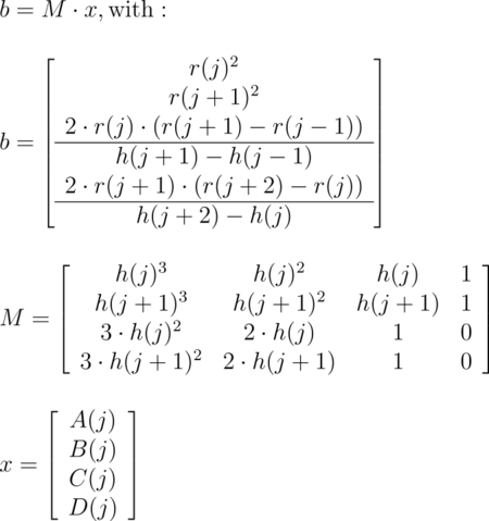
|
|
Curve Math |
where r(j) is the radius and h(j) is the height of point P(j).
The figure below shows the configuration of the points P(i), the location of segment j, and the curve that is defined by this segment.
|
|
Points on a surface of revolution. |
3.4.5.1.16 Text
A text object creates 3-D text as an extruded block letter. Currently only TrueType fonts (ttf) and TrueType Collections (ttc) are supported but the syntax allows for other font types to be added in the future. If TrueType Collections are used, the first font found in the collection will be used. The syntax is:
TEXT_OBECT:
  text {
    ttf "fontname.ttf/ttc" "String_of_Text"
    Thickness, <Offset>
    [OBJECT_MODIFIERS...]
    }
Where fontname.ttf or fontname.ttc is the name of the TrueType font file. It is a quoted string literal or string expression. The string expression which follows is the actual text of the string object. It too may be a quoted string literal or string expression. See section Strings for more on string expressions.
In version 3.7 several fonts are now built-in. It should be noted that this is only a preliminary solution so the benchmark program will run without installing POV-Ray. Future versions may lack this mechanism, so in scene files (other than the built-in benchmark) you should continue to reference the external font files as before. Consequently, the following alternate syntax is available:
TEXT_OBECT:
  text {
    internal Font_Number "String_of_Text"
    Thickness, <Offset>
    [OBJECT_MODIFIERS] }
    }
Where Font_Number is one of the integer values from the list below:
- povlogo.ttf
- timrom.ttf
- cyrvetic.ttf
- crystal.ttf
Note: An out of range Font_Number value will default to 0.
The text will start with the origin at the lower left, front of the first character and will extend in the +x-direction. The baseline of the text follows the x-axis and descender drop into the -y-direction. The front of the character sits in the x-y-plane and the text is extruded in the +z-direction. The front-to-back thickness is specified by the required value
Thickness.
Characters are generally sized so that 1 unit of vertical spacing is correct. The characters are about 0.5 to 0.75 units tall.
The horizontal spacing is handled by POV-Ray internally including any kerning information stored in the font. The required vector <Offset> defines any extra translation between each character. Normally you should specify a zero for this value. Specifying 0.1*x would put additional 0.1 units of space between each character. Here is an example:
text {
  ttf "timrom.ttf" "POV-Ray" 1, 0
  pigment { Red }
  }
Only printable characters are allowed in text objects. Characters such as return, line feed, tabs, backspace etc. are not supported.
For easy access to your fonts, set the Library_Path to the directory that contains your font collection.
3.4.5.1.17 Torus
A torus is a 4th order quartic polynomial shape that looks
like a donut or inner tube. Because this shape is so useful and quartics are
difficult to define, POV-Ray lets you take a short-cut and define a torus
by:
TORUS:
  torus {
    Major, Minor
    [TORUS_MODIFIER...]
    }
TORUS_MODIFIER:
  sturm | OBJECT_MODIFIER
Torus default values:
sturm : off
where Major is a float value giving the major radius
and Minor is a float specifying the minor radius. The
major radius extends from the center of the hole to the mid-line of the rim
while the minor radius is the radius of the cross-section of the rim. The
torus is centered at the origin and lies in the x-z-plane with the y-axis
sticking through the hole.
|
|
Major and minor radius of a torus. |
The torus is internally bounded by two cylinders and two rings forming a thick cylinder. With this bounding cylinder the performance of the torus intersection test is vastly increased. The test for a valid torus intersection, i.e. solving a 4th order polynomial, is only performed if the bounding cylinder is hit. Thus a lot of slow root solving calculations are avoided.
Calculations for all higher order polynomials must be very accurate. If the
torus renders improperly you may add the keyword sturm to use
POV-Ray's slower-yet-more-accurate Sturmian root solver.
3.4.5.2 Finite Patch Primitives
There are six totally thin, finite objects which have no well-defined inside. They are bicubic patch, disc, smooth triangle, triangle, polygon, mesh, and mesh2. They may be combined in CSG union, but cannot be used inside a clipped_by statement.
Note: Patch objects may give unexpected results when used in differences and intersections.
These conditions apply:
- Solids may be differenced from bicubic patches with the expected results.
- Differencing a bicubic patch from a solid may give unexpected results.
- Especially if the inverse keyword is used!
- Intersecting a solid and a bicubic patch will give the expected results.
- The parts of the patch that intersect the solid object will be visible.
- Merging a solid and a bicubic patch will remove the parts of the bicubic patch that intersect the solid.
Because these types are finite POV-Ray can use automatic bounding on them to speed up rendering time. As with all shapes they can be translated, rotated and scaled.
3.4.5.2.1 Bicubic Patch
A bicubic_patch is a 3D curved surface created from a mesh of
triangles. POV-Ray supports a type of bicubic patch called a Bezier
patch. A bicubic patch is defined as follows:
BICUBIC_PATCH:
  bicubic_patch {
    PATCH_ITEMS...
    <Point_1>,<Point_2>,<Point_3>,<Point_4>,
    <Point_5>,<Point_6>,<Point_7>,<Point_8>,
    <Point_9>,<Point_10>,<Point_11>,<Point_12>,
    <Point_13>,<Point_14>,<Point_15>,<Point_16>
    [OBJECT_MODIFIERS...]
    }
PATCH_ITEMS:
  type Patch_Type | u_steps Num_U_Steps | v_steps Num_V_Steps |
  flatness Flatness
Bicubic patch default values:
flatness : 0.0
u_steps  : 0
v_steps  : 0
The keyword type is followed by a float
Patch_Type which currently must be either 0 or 1. For type 0 only
the control points are retained within POV-Ray. This means that a minimal
amount of memory is needed but POV-Ray will need to perform many extra
calculations when trying to render the patch. Type 1 preprocesses the patch
into many subpatches. This results in a significant speedup in rendering at
the cost of memory.
The four parameters type, flatness,
u_steps and v_steps may appear in any order. Only
type is required. They are followed by 16 vectors (4 rows
of 4) that define the x, y, z coordinates of the 16 control points which
define the patch. The patch touches the four corner points
<Point_1>, <Point_4>,
<Point_13> and
<Point_16> while the other 12 points pull and stretch the
patch into shape. The Bezier surface is enclosed by the convex hull formed by
the 16 control points, this is known as the convex hull property.
The keywords u_steps and v_steps are each followed
by integer values which tell how many rows and columns of triangles are the
minimum to use to create the surface, both default to 0. The maximum number of individual pieces
of the patch that are tested by POV-Ray can be calculated from the following:
pieces = 2^u_steps * 2^v_steps.
This means that you really should keep u_steps and
v_steps under 4. Most patches look just fine with u_steps
3 and v_steps 3, which translates to 64 sub-patches (128
smooth triangles).
As POV-Ray processes the Bezier patch it makes a test of the current piece
of the patch to see if it is flat enough to just pretend it is a rectangle.
The statement that controls this test is specified with the
flatness keyword followed by a float. Typical flatness values range
from 0 to 1 (the lower the slower). The default if none is specified is
0.0.
If the value for flatness is 0 POV-Ray will always subdivide the patch to
the extend specified by u_steps and v_steps. If
flatness is greater than 0 then every time the patch is split, POV-Ray will
check to see if there is any need to split further.
There are both advantages and disadvantages to using a non-zero flatness. The advantages include:
- If the patch is not very curved, then this will be detected and POV-Ray will not waste a lot of time looking at the wrong pieces.
- If the patch is only highly curved in a couple of places, POV-Ray will keep subdividing there and concentrate its efforts on the hard part.
The biggest disadvantage is that if POV-Ray stops subdividing at a particular level on one part of the patch and at a different level on an adjacent part of the patch there is the potential for cracking. This is typically visible as spots within the patch where you can see through. How bad this appears depends very highly on the angle at which you are viewing the patch.
Like triangles, the bicubic patch is not meant to be generated by hand. These shapes should be created by a special utility. You may be able to acquire utilities to generate these shapes from the same source from which you obtained POV-Ray. Here is an example:
bicubic_patch {
  type 0
  flatness 0.01
  u_steps 4
  v_steps 4
  <0, 0, 2>, <1, 0, 0>, <2, 0, 0>, <3, 0,-2>,
  <0, 1  0>, <1, 1, 0>, <2, 1, 0>, <3, 1, 0>,
  <0, 2, 0>, <1, 2, 0>, <2, 2, 0>, <3, 2, 0>,
  <0, 3, 2>, <1, 3, 0>, <2, 3, 0>, <3, 3, -2>
  }
The triangles in a POV-Ray bicubic_patch are automatically
smoothed using normal interpolation but it is up to the user (or the
user's utility program) to create control points which smoothly stitch
together groups of patches.
3.4.5.2.2 Disc
Another flat, finite object available with POV-Ray is the
disc. The disc is infinitely thin, it has no thickness. If you want a
disc with true thickness you should use a very short cylinder. A disc shape
may be defined by:
DISC:
  disc {
    <Center>, <Normal>, Radius [, Hole_Radius]
    [OBJECT_MODIFIERS...]
    }
Disc default values:
HOLE RADIUS : 0.0
The vector <Center> defines the x, y, z
coordinates of the center of the disc. The
<Normal> vector describes its orientation by describing its
surface normal vector. This is followed by a float specifying the
Radius. This may be optionally followed by another float
specifying the radius of a hole to be cut from the center of the disc.
Note: The inside of a disc is the inside of the plane that contains the disc. Also note that it is not constrained by the radius of the disc.
3.4.5.2.3 Mesh
The mesh object can be used to efficiently store large
numbers of triangles. Its syntax is:
MESH:
  mesh {
    MESH_TRIANGLE...
    [MESH_MODIFIER...]
    }
MESH_TRIANGLE:
  triangle {
    <Corner_1>, <Corner_2>, <Corner_3>
    [uv_vectors <uv_Corner_1>, <uv_Corner_2>, <uv_Corner_3>]
    [MESH_TEXTURE]
    } |

  smooth_triangle {
    <Corner_1>, <Normal_1>,
    <Corner_2>, <Normal_2>,
    <Corner_3>, <Normal_3>
    [uv_vectors <uv_Corner_1>, <uv_Corner_2>, <uv_Corner_3>]
    [MESH_TEXTURE]
    }
MESH_TEXTURE:
  texture { TEXTURE_IDENTIFIER }
  texture_list {
    TEXTURE_IDENTIFIER TEXTURE_IDENTIFIER TEXTURE_IDENTIFIER
    }

MESH_MODIFIER:
  inside_vector <direction> | hierarchy [ Boolean ] |
  OBJECT_MODIFIER
Mesh default values:
hierarchy : on
Any number of triangle and/or smooth_triangle
statements can be used and each of those triangles can be individually
textured by assigning a texture identifier to it. The texture has to be
declared before the mesh is parsed. It is not possible to use texture
definitions inside the triangle or smooth triangle statements. This is a
restriction that is necessary for an efficient storage of the assigned
textures. See Triangle and Smooth Triangle for more information on triangles.
The mesh object can support uv_mapping. For this, per triangle the keyword
uv_vectors has to be given, together with three 2D uv-vectors. Each vector specifies a location
in the xy-plane from which the texture has to be mapped to the matching points of the triangle.
Also see the section uv_mapping.
The mesh's components are internally bounded by a bounding box hierarchy
to speed up intersection testing. The bounding hierarchy can be turned off
with the hierarchy off keyword. This should only be done if
memory is short or the mesh consists of only a few triangles. The default is
hierarchy on.
Copies of a mesh object refer to the same triangle data and thus consume very little memory. You can easily trace a hundred copies of a 10000 triangle mesh without running out of memory (assuming the first mesh fits into memory). The mesh object has two advantages over a union of triangles: it needs less memory and it is transformed faster. The memory requirements are reduced by efficiently storing the triangles vertices and normals. The parsing time for transformed meshes is reduced because only the mesh object has to be transformed and not every single triangle as it is necessary for unions.
The mesh object can currently only include triangle and smooth triangle components. That restriction may change, allowing polygonal components, at some point in the future.
3.4.5.2.3.1 Solid Mesh
The triangle mesh objects mesh (and mesh2) can be used in CSG objects such as difference and intersect. Adding the inside_vector they do have a defined inside. This will only work for well-behaved meshes, which are completely closed volumes. If meshes have any holes in them, this might work, but the results are not guaranteed.
To determine if a point is inside a triangle mesh, POV-Ray shoots a ray from the point in some arbitrary direction. If this vector intersects an odd number of triangles, the point is inside the mesh. If it intersects an even number of triangles, the point is outside of the mesh. You can specify the direction of this vector. For example, to use +z as the direction, you would add the following line to the triangle mesh description (following all other mesh data, but before the object modifiers).
inside_vector <0, 0, 1>
This change does not have any effect on unions of triangles, these will still be always hollow.
3.4.5.2.4 Mesh2
The new mesh syntax is designed for use in conversion from other file formats.
MESH2 :
  mesh2{
    VECTORS...
    LISTS...   |
    INDICES... |
    MESH_MODIFIERS
    }
VECTORS :
  vertex_vectors {
  number_of_vertices,
  <vertex1>, <vertex2>, ...
  }|
  normal_vectors {
    number_of_normals,
    <normal1>, <normal2>, ...
    }|
  uv_vectors {
    number_of_uv_vectors,
    <uv_vect1>, <uv_vect2>, ...
    }
LISTS :
  texture_list {
    number_of_textures,
    texture { Texture1 },
    texture { Texture2 }, ...
    }|
INDICES :
  face_indices {
    number_of_faces,
      <index_a, index_b, index_c> [,texture_index [,
    texture_index, texture_index]],
      <index_d, index_e, index_f> [,texture_index [,
      texture_index, texture_index]],
      ...
      }|
  normal_indices {
    number_of_faces,
      <index_a, index_b, index_c>,
      <index_d, index_e, index_f>,
      ...
      }|
  uv_indices {
    number_of_faces,
      <index_a, index_b, index_c>,
      <index_d, index_e, index_f>,
      ...
      }
MESH_MODIFIER :
  inside_vector <direction> | OBJECT_MODIFIERS
The mesh2 object definition MUST be specified in the following order:
- VECTORS
- LISTS
- INDICES
The normal_vectors, uv_vectors, and texture_list sections are optional.
If the number of normals equals the number of vertices then the normal_indices section is optional and the indexes from the face_indices section are used instead. Likewise for the uv_indices section.
Note: The texture_list section is optional only if face_indices doesn't contain any texture index values.
For example:
face_indices {
  number_of_faces,
  <index_a, index_b, index_c>,
  <index_d, index_e, index_f>,
  ...
  }
Note: The numbers of uv_indices must equal number of faces.
The indexes are zero based, so the first item in each list has an index of zero.
3.4.5.2.4.1 Smooth and Flat triangles in the same mesh
You can specify both flat and smooth triangles in the same mesh. To do this, specify
the smooth triangles first in the face_indices
section, followed by the flat triangles. Then, specify normal indices (in the
normal_indices section) for only the
smooth triangles. Any remaining triangles that do not have normal indices associated with
them will be assumed to be flat triangles.
3.4.5.2.4.2 Mesh Triangle Textures
To specify a texture for an individual mesh triangle, specify a single integer texture index following the face-index vector for that triangle.
To specify three textures for vertex-texture interpolation, specify three integer texture indices (separated by commas) following the face-index vector for that triangle.
Vertex-texture interpolation and textures for an individual triangle can be mixed in the same mesh.
3.4.5.2.5 Polygon
The polygon object is useful for creating rectangles, squares
and other planar shapes with more than three edges. Their syntax is:
POLYGON:
  polygon {
    Number_Of_Points, <Point_1> <Point_2>... <Point_n>
    [OBJECT_MODIFIER...]
    }
The float Number_Of_Points tells how many points are
used to define the polygon. The points <Point_1>
through <Point_n> describe the polygon or
polygons. A polygon can contain any number of sub-polygons, either
overlapping or not. In places where an even number of polygons overlaps a
hole appears. When you repeat the first point of a sub-polygon, it closes it
and starts a new sub-polygon's point sequence. This means that all points
of a sub-polygon are different.
If the last sub-polygon is not closed a warning is issued and the program automatically closes the polygon. This is useful because polygons imported from other programs may not be closed, i.e. their first and last point are not the same.
All points of a polygon are three-dimensional vectors that have to lay on the same plane. If this is not the case an error occurs. It is common to use two-dimensional vectors to describe the polygon. POV-Ray assumes that the z value is zero in this case.
A square polygon that matches the default planar image map is simply:
polygon {
  4,
  <0, 0>, <0, 1>, <1, 1>, <1, 0>
  texture {
    finish { ambient 1 diffuse 0 }
    pigment { image_map { gif "test.gif"  } }
    }
  //scale and rotate as needed here
  }
The sub-polygon feature can be used to generate complex shapes like the letter "P", where a hole is cut into another polygon:
#declare P = polygon {
  12,
  <0, 0>, <0, 6>, <4, 6>, <4, 3>, <1, 3>, <1,0>, <0, 0>,
  <1, 4>, <1, 5>, <3, 5>, <3, 4>, <1, 4>
  }
The first sub-polygon (on the first line) describes the outer shape of the letter "P". The second sub-polygon (on the second line) describes the rectangular hole that is cut in the top of the letter "P". Both rectangles are closed, i.e. their first and last points are the same.
The feature of cutting holes into a polygon is based on the polygon inside/outside test used. A point is considered to be inside a polygon if a straight line drawn from this point in an arbitrary direction crosses an odd number of edges, this is known as Jordan's curve theorem.
Another very complex example showing one large triangle with three small holes and three separate, small triangles is given below:
polygon {
  28,
  <0, 0> <1, 0> <0, 1> <0, 0>          // large outer triangle
  <.3, .7> <.4, .7> <.3, .8> <.3, .7>  // small outer triangle #1
  <.5, .5> <.6, .5> <.5, .6> <.5, .5>  // small outer triangle #2
  <.7, .3> <.8, .3> <.7, .4> <.7, .3>  // small outer triangle #3
  <.5, .2> <.6, .2> <.5, .3> <.5, .2>  // inner triangle #1
  <.2, .5> <.3, .5> <.2, .6> <.2, .5>  // inner triangle #2
  <.1, .1> <.2, .1> <.1, .2> <.1, .1>  // inner triangle #3
  }
3.4.5.2.6 Triangle
The triangle primitive is available in order to make more
complex objects than the built-in shapes will permit. Triangles are usually
not created by hand but are converted from other files or generated by
utilities. A triangle is defined by
TRIANGLE:
  triangle {
    <Corner_1>, <Corner_2>, <Corner_3>
    [OBJECT_MODIFIER...]
    }
where <Corner_n> is a vector defining the x,
y, z coordinates of each corner of the triangle.
Because triangles are perfectly flat surfaces it would require extremely large numbers of very small triangles to approximate a smooth, curved surface. However much of our perception of smooth surfaces is dependent upon the way light and shading is done. By artificially modifying the surface normals we can simulate a smooth surface and hide the sharp-edged seams between individual triangles.
3.4.5.2.7 Smooth Triangle
The smooth_triangle primitive is used for just such purposes.
The smooth triangles use a formula called Phong normal interpolation to
calculate the surface normal for any point on the triangle based on normal
vectors which you define for the three corners. This makes the triangle
appear to be a smooth curved surface. A smooth triangle is defined by
SMOOTH_TRIANGLE:
  smooth_triangle {
  <Corner_1>, <Normal_1>, <Corner_2>,
  <Normal_2>, <Corner_3>, <Normal_3>
  [OBJECT_MODIFIER...]
  }
where the corners are defined as in regular triangles and
<Normal_n> is a vector describing the direction of the
surface normal at each corner.
These normal vectors are prohibitively difficult to compute by hand. Therefore smooth triangles are almost always generated by utility programs. To achieve smooth results, any triangles which share a common vertex should have the same normal vector at that vertex. Generally the smoothed normal should be the average of all the actual normals of the triangles which share that point.
The mesh object is a way to combine many triangle
and smooth_triangle objects together in a very efficient way.
See Mesh for details.
3.4.5.3 Infinite Solid Primitives
There are six polynomial primitive shapes that are possibly infinite and
do not respond to automatic bounding. They are plane, cubic, poly, quartic, polynomial,
and quadric. They do have a well defined inside and may be used in CSG and
inside a clipped_by statement. As with all shapes they can be
translated, rotated and scaled.
3.4.5.3.1 Plane
The plane primitive is a simple way to define an infinite
flat surface. The plane is not a thin boundary or can be compared to a sheet
of paper. A plane is a solid object of infinite size that divides POV-space
in two parts, inside and outside the plane. The plane is specified as follows:
PLANE:
  plane {
    <Normal>, Distance
    [OBJECT_MODIFIERS...]
    }
The <Normal> vector defines the surface normal
of the plane. A surface normal is a vector which points up from the surface
at a 90 degree angle. This is followed by a float value that gives the
distance along the normal that the plane is from the origin (that is only
true if the normal vector has unit length; see below). For example:
plane { <0, 1, 0>, 4 }
This is a plane where straight up is defined in the positive y-direction.
The plane is 4 units in that direction away from the origin. Because most
planes are defined with surface normals in the direction of an axis you will
often see planes defined using the x, y or
z built-in vector identifiers. The example above could be specified
as:
plane { y, 4 }
The plane extends infinitely in the x- and z-directions. It effectively
divides the world into two pieces. By definition the normal vector points to
the outside of the plane while any points away from the vector are defined as
inside. This inside/outside distinction is important when using planes in CSG
and clipped_by. It is also important when using fog or
atmospheric media. If you place a camera on the "inside" half of
the world, then the fog or media will not appear. Such issues arise in any
solid object but it is more common with planes. Users typically know when
they have accidentally placed a camera inside a sphere or box but
"inside a plane" is an unusual concept. In general you can reverse the
inside/outside properties of an object by adding the object modifier
inverse. See Inverse and Empty and Solid Objects for details.
A plane is called a polynomial shape because it is defined by a first order polynomial equation. Given a plane:
plane { <A, B, C>, D }
it can be represented by the equation A*x + B*y + C*z - D*sqrt(A^2 + B^2 + C^2) = 0.
Therefore our example plane{y,4} is actually the polynomial
equation y=4. You can think of this as a set of all x, y, z points where all
have y values equal to 4, regardless of the x or z values.
This equation is a first order polynomial because each term contains only single powers of x, y or z. A second order equation has terms like x^2, y^2, z^2, xy, xz and yz. Another name for a 2nd order equation is a quadric equation. Third order polys are called cubics. A 4th order equation is a quartic. Such shapes are described in the sections below.
3.4.5.3.2 Poly
Higher order polynomial surfaces may be defined by the use of a
poly shape. The syntax is
POLY:
  poly {
    Order, <A1, A2, A3,... An>
    [POLY_MODIFIERS...]
    }
POLY_MODIFIERS:
  sturm | OBJECT_MODIFIER
Poly default values:
sturm : off
where Order is an integer number from 2 to 35
inclusively that specifies the order of the equation. A1, A2, ...
An are float values for the coefficients of the equation. There
are n such terms where n = ((Order+1)*(Order+2)*(Order+3))/6.
3.4.5.3.3 Cubic
The cubic object
is an alternate way to specify 3rd order polys. Its syntax is:
CUBIC:
  cubic {
    <A1, A2, A3,... A20>
    [POLY_MODIFIERS...]
    }
3.4.5.3.4 Quartic
Also 4th order equations may be specified with the quartic
object. Its syntax is:
QUARTIC:
  quartic {
    <A1, A2, A3,... A35>
    [POLY_MODIFIERS...]
    }
3.4.5.3.5 Polynomial
Poly, cubic and quartics are just like quadrics in that you do not have
to understand one to use one. The file shapesq.inc has
plenty of pre-defined quartics for you to play with.
For convenience an alternate syntax is available as polynomial. It doesn't care about the order of the coefficients, as long as you do not define them more than once, otherwise only the value of the last definition is kept. Additionally the default with all coefficients is 0, which can be especially useful typing shortcut.
See the tutorial section for more examples of the simplified syntax.
POLYNOMIAL:
  polynomial {
    Order, [COEFFICIENTS...]
    [POLY_MODIFIERS...]
    }
COEFFICIENTS:
  xyz(<x_power>,<y_power>,<z_power>):<value>[,]
POLY_MODIFIERS:
  sturm | OBJECT_MODIFIER
Same as the torus above, but with the polynomial syntax:
// Torus having major radius sqrt(40), minor radius sqrt(12)
polynomial { 4,
  xyz(4,0,0):1,
  xyz(2,2,0):2,
  xyz(2,0,2):2,
  xyz(2,0,0):-104,
  xyz(0,4,0):1,
  xyz(0,2,2):2,
  xyz(0,2,0):56,
  xyz(0,0,4):1,
  xyz(0,0,2):-104,
  xyz(0,0,0):784
  sturm
  }
The following table shows which polynomial terms correspond to which x,y,z
factors for the orders 2 to 7. Remember cubic is actually a 3rd order polynomial and
quartic is 4th order.
| 2nd | 3rd | 4th | 5th | 6th | 7th | 5th | 6th | 7th | 6th | 7th | |||
|---|---|---|---|---|---|---|---|---|---|---|---|---|---|
| A1 | x2 | x3 | x4 | x5 | x6 | x7 | A41 | y3 | xy3 | x2y3 | A81 | z3 | xz3 |
| A2 | xy | x2y | x3y | x4y | x5y | x6y | A42 | y2z3 | xy2z3 | x2y2z3 | A82 | z2 | xz2 |
| A3 | xz | x2z | x3z | x4z | x5z | x6z | A43 | y2z2 | xy2z2 | x2y2z2 | A83 | z | xz |
| A4 | x | x2 | x3 | x4 | x5 | x6 | A44 | y2z | xy2z | x2y2z | A84 | 1 | x |
| A5 | y2 | xy2 | x2y2 | x3y2 | x4y2 | x5y2 | A45 | y2 | xy2 | x2y2 | A85 | y7 | |
| A6 | yz | xyz | x2yz | x3yz | x4yz | x5yz | A46 | yz4 | xyz4 | x2yz4 | A86 | y6z | |
| A7 | y | xy | x2y | x3y | x4y | x5y | A47 | yz3 | xyz3 | x2yz3 | A87 | y6 | |
| A8 | z2 | xz2 | x2z2 | x3z2 | x4z2 | x5z2 | A48 | yz2 | xyz2 | x2yz2 | A88 | y5z2 | |
| A9 | z | xz | x2z | x3z | x4z | x5z | A49 | yz | xyz | x2yz | A89 | y5z | |
| A10 | 1 | x | x2 | x3 | x4 | x5 | A50 | y | xy | x2y | A90 | y5 | |
| A11 | y3 | xy3 | x2y3 | x3y3 | x4y3 | A51 | z5 | xz5 | x2z5 | A91 | y4z3 | ||
| A12 | y2z | xy2z | x2y2z | x3y2z | x4y2z | A52 | z4 | xz4 | x2z4 | A92 | y4z2 | ||
| A13 | y2 | xy2 | x2y2 | x3y2 | x4y2 | A53 | z3 | xz3 | x2z3 | A93 | y4z | ||
| A14 | yz2 | xyz2 | x2yz2 | x3yz2 | x4yz2 | A54 | z2 | xz2 | x2z2 | A94 | y4 | ||
| A15 | yz | xyz | x2yz | x3yz | x4yz | A55 | z | xz | x2z | A95 | y3z4 | ||
| A16 | y | xy | x2y | x3y | x4y | A56 | 1 | x | x2 | A96 | y3z3 | ||
| A17 | z3 | xz3 | x2z3 | x3z3 | x4z3 | A57 | y6 | xy6 | A97 | y3z2 | |||
| A18 | z2 | xz2 | x2z2 | x3z2 | x4z2 | A58 | y5z | xy5z | A98 | y3z | |||
| A19 | z | xz | x2z | x3z | x4z | A59 | y5 | xy5 | A99 | y3 | |||
| A20 | 1 | x | x2 | x3 | x4 | A60 | y4z2 | xy4z2 | A100 | y2z5 | |||
| A21 | y4 | xy4 | x2y4 | x3y4 | A61 | y4z | xy4z | A101 | y2z4 | ||||
| A22 | y3z | xy3z | x2y3z | x3y3z | A62 | y4 | xy4 | A102 | y2z3 | ||||
| A23 | y3 | xy3 | x2y3 | x3y3 | A63 | y3z3 | xy3z3 | A103 | y2z2 | ||||
| A24 | y2z2 | xy2z2 | x2y2z2 | x3y2z2 | A64 | y3z2 | xy3z2 | A104 | y2z | ||||
| A25 | y2z | xy2z | x2y2z | x3y2z | A65 | y3z | xy3z | A105 | y2 | ||||
| A26 | y2 | xy2 | x2y2 | x3y2 | A66 | y3 | xy3 | A106 | yz6 | ||||
| A27 | yz3 | xyz3 | x2yz3 | x3yz3 | A67 | y2z4 | xy2z4 | A107 | yz5 | ||||
| A28 | yz2 | xyz2 | x2yz2 | x3yz2 | A68 | y2z3 | xy2z3 | A108 | yz4 | ||||
| A29 | yz | xyz | x2yz | x3yz | A69 | y2z2 | xy2z2 | A109 | yz3 | ||||
| A30 | y | xy | x2y | x3y | A70 | y2z | xy2z | A110 | yz2 | ||||
| A31 | z4 | xz4 | x2z4 | x3z4 | A71 | y2 | xy2 | A111 | yz | ||||
| A32 | z3 | xz3 | x2z3 | x3z3 | A72 | yz5 | xyz5 | A112 | y | ||||
| A33 | z2 | xz2 | x2z2 | x3z2 | A73 | yz4 | xyz4 | A113 | z7 | ||||
| A34 | z | xz | x2z | x3z | A74 | yz3 | xyz3 | A114 | z6 | ||||
| A35 | 1 | x | x2 | x3 | A75 | yz2 | xyz2 | A115 | z5 | ||||
| A36 | y5 | xy5 | x2y5 | A76 | yz | xyz | A116 | z4 | |||||
| A37 | y4z | xy4z | x2y4z | A77 | y | xy | A117 | z3 | |||||
| A38 | y4 | xy4 | x2y4 | A78 | z6 | xz6 | A118 | z2 | |||||
| A39 | y3z2 | xy3z2 | x2y3z2 | A79 | z5 | xz5 | A119 | z | |||||
| A40 | y3z | xy3z | x2y3z | A80 | z4 | xz4 | A120 | 1 |
Polynomial shapes can be used to describe a large class of shapes
including the torus, the lemniscate, etc. For example, to declare a quartic
surface requires that each of the coefficients (A1 ...
A35) be placed in order into a single long vector of 35 terms. As an example let's define a torus the hard way. A Torus can be represented by the equation: x4 + y4 + z4 + 2 x2 y2 + 2 x2 z2 + 2 y2 z2 - 2 (r_02 + r_12)
x2 + 2 (r_02 - r_12) y2 - 2 (r_02 + r_12) z2 + (r_02 - r_12)2 = 0
Where r_0 is the major radius of the torus, the distance from the hole of the donut to the middle of the ring of the donut, and r_1 is the minor radius of the torus, the distance from the middle of the ring of the donut to the outer surface. The following object declaration is for a torus having major radius 6.3 minor radius 3.5 (Making the maximum width just under 20).
// Torus having major radius sqrt(40), minor radius sqrt(12)
quartic {
  < 1,   0,   0,   0,   2,   0,   0,   2,   0,
  -104,   0,   0,   0,   0,   0,   0,   0,   0,
  0,   0,   1,   0,   0,   2,   0,  56,   0,
  0,   0,   0,   1,   0, -104,  0, 784 >
  sturm
  }
Polynomial surfaces use highly complex computations and will not always render perfectly.
If the surface is not smooth, has dropouts, or extra random pixels, try using
the optional keyword sturm in the definition. This will cause a
slower but more accurate calculation method to be used. Usually, but not
always, this will solve the problem. If sturm does not work, try rotating
or translating the shape by some small amount.
There are really so many different polynomial shapes, we cannot even begin to list or describe them all. We suggest you find a good reference or text book if you want to investigate the subject further.
3.4.5.3.6 Quadric
The quadric object can produce shapes like paraboloids (dish
shapes) and hyperboloids (saddle or hourglass shapes). It can also produce
ellipsoids, spheres, cones, and cylinders but you should use the
sphere, cone, and cylinder objects built
into POV-Ray because they are faster than the quadric version.
Note: Do not confuse "quaDRic" with "quaRTic". A quadric is a 2nd order polynomial while a quartic is 4th order.
Quadrics render much faster and are less error-prone but produce less complex objects. The syntax is:
QUADRIC:
  quadric {
    <A,B,C>,<D,E,F>,<G,H,I>,J
    [OBJECT_MODIFIERS...]
    }
Although the syntax actually will parse 3 vector expressions followed by a
float, we traditionally have written the syntax as above where
A through J are float expressions. These 10
float that define a surface of x, y, z points which satisfy the equation A x2
+ B y2 + C z2 + D xy + E xz + F yz + G x + H y + I z + J = 0
Different values of A, B, C, ... J will give
different shapes. If you take any three dimensional point and use its x, y
and z coordinates in the above equation the answer will be 0 if the point is
on the surface of the object. The answer will be negative if the point is
inside the object and positive if the point is outside the object. Here are
some examples:
| X2 + Y2 + Z2 - 1 = 0 | Sphere |
| X2 + Y2 - 1 = 0 | Infinite cylinder along the Z axis |
| X2 + Y2 - Z2 = 0 | Infinite cone along the Z axis |
The easiest way to use these shapes is to include the standard file
shapes.inc into your program. It contains several pre-defined quadrics
and you can transform these pre-defined shapes (using translate, rotate and
scale) into the ones you want. For a complete list, see the file
shapes.inc.
3.4.5.4 Constructive Solid Geometry
In addition to all of the primitive shapes POV-Ray supports, you can also combine multiple simple shapes into complex shapes using Constructive Solid Geometry (CSG). There are four basic types of CSG operations: union, intersection, difference, and merge. CSG objects can be composed of primitives or other CSG objects to create more, and more complex shapes.
3.4.5.4.1 Inside and Outside
Most shape primitives, like spheres, boxes and blobs divide the world into two regions. One region is inside the object and one is outside. Given any point in space you can say it is either inside or outside any particular primitive object. Well, it could be exactly on the surface but this case is rather hard to determine due to numerical problems.
Even planes have an inside and an outside. By definition, the surface normal
of the plane points towards the outside of the plane. You should note that
triangles cannot be used as solid objects in CSG since they have no well defined inside and outside. Triangle-based shapes (mesh and mesh2) can only be used in CSG when they are closed objects and have an inside vector specified.
Note: Although the triangle, the bicubic_patch and some other shapes have no well defined inside and outside, they have a front- and backside which makes it possible to use a texture on the front side and an interior_texture on the back side.
CSG uses the concepts of inside and outside to combine shapes together as explained in the following sections.
Imagine you have two objects that partially overlap like shown in the figure
below. Four different areas of points can be distinguished: points that are
neither in object A nor in object B, points that
are in object A but not in object B, points that
are not in object A but in object B and last not
least points that are in object A and object B.
|
|
Two overlapping objects. |
Keeping this in mind it will be quite easy to understand how the CSG operations work.
When using CSG it is often useful to invert an object so that it will be
inside-out. The appearance of the object is not changed, just the way that
POV-Ray perceives it. When the inverse keyword is used the
inside of the shape is flipped to become the outside and vice
versa.
The inside/outside distinction is not important for a union, but is important for intersection, difference, and merge. Therefore any objects may be combined using union but only solid objects, i.e. objects that have a well-defined interior can be used in the other kinds of CSG. The objects described in
Finite Patch Primitives have no well defined inside/outside. All objects described in the sections Finite Solid Primitives and Infinite Solid Primitives.
3.4.5.4.2 Union
|
|
The union of two objects. |
The simplest kind of CSG is the union. The syntax is:
UNION:
  union {
    OBJECTS...
    [OBJECT_MODIFIERS...]
    }
Unions are simply glue used to bind two or more shapes into a single
entity that can be manipulated as a single object. The image above shows the
union of A and B. The new object created by the
union operation can be scaled, translated and rotated as a single shape. The
entire union can share a single texture but each object contained in the
union may also have its own texture, which will override any texture
statements in the parent object.
You should be aware that the surfaces inside the union will not be removed.
As you can see from the figure this may be a problem for transparent unions.
If you want those surfaces to be removed you will have to use the
merge operations explained in a later section.
The following union will contain a box and a sphere.
union {
  box { <-1.5, -1, -1>, <0.5, 1, 1> }
  cylinder { <0.5, 0, -1>, <0.5, 0, 1>, 1 }
  }
Earlier versions of POV-Ray placed restrictions on unions so you often had
to combine objects with composite statements. Those earlier
restrictions have been lifted so composite is no longer needed.
It is still supported for backwards compatibility.
3.4.5.4.2.1 Split_Union
split_union is a boolean keyword that can be added to a union.
It has two states on/off, its default is on.
split_union is used when photons are shot
at the CSG-object. The object is split up in its compound parts, photons are shot at
each part separately. This is to prevent photons from being shot at 'empty spaces' in the object,
for example the holes in a grid. With compact objects, without 'empty spaces'
split_union off can improve photon
gathering.
union {
  object {...}
  object {...}
  split_union off
  }
3.4.5.4.3 Intersection
The intersection object creates a shape containing only those
areas where all components overlap. A point is part of an intersection if it is
inside both objects, A and B, as show in the figure
below.
|
|
The intersection of two objects. |
The syntax is:
INTERSECTION:
  intersection {
    SOLID_OBJECTS...
    [OBJECT_MODIFIERS...]
    }
The component objects must have well defined inside/outside properties. Patch objects are not allowed.
Note: If all components do not overlap, the intersection object disappears.
Here is an example that overlaps:
intersection {
  box { <-1.5, -1, -1>, <0.5, 1, 1> }
  cylinder { <0.5, 0, -1>, <0.5, 0, 1>, 1 }
  }
3.4.5.4.4 Difference
The CSG difference operation takes the intersection between
the first object and the inverse of all subsequent objects. Thus only points
inside object A and outside object B belong to the
difference of both objects.
The result is a subtraction of the 2nd shape from the first shape as shown in the figure below.
|
|
The difference between two objects. |
The syntax is:
DIFFERENCE:
  difference {
    SOLID_OBJECTS...
    [OBJECT_MODIFIERS...]
    }
The component objects must have well defined inside/outside properties. Patch objects are not allowed.
Note: If the first object is entirely inside the subtracted objects, the difference object disappears.
Here is an example of a properly formed difference:
difference {
  box { <-1.5, -1, -1>, <0.5, 1, 1> }
  cylinder { <0.5, 0, -1>, <0.5, 0, 1>, 1 }
  }
Note: Internally, POV-Ray simply adds the inverse keyword
to the second (and subsequent) objects and then performs an intersection.
The example above is equivalent to:
intersection {
  box { <-1.5, -1, -1>, <0.5, 1, 1> }
  cylinder { <0.5, 0, -1>, <0.5, 0, 1>, 1 inverse }
  }
3.4.5.4.5 Merge
The union operation just glues objects together, it does not
remove the objects' surfaces inside the union. Under most
circumstances this does not matter. However if a transparent
union is used, those interior surfaces will be visible. The
merge operations can be used to avoid this problem. It works just like
union but it eliminates the inner surfaces like shown in the
figure below.

|
|
Merge removes inner surfaces. |
The syntax is:
MERGE:
  merge {
    SOLID_OBJECTS...
    [OBJECT_MODIFIERS...]
    }
The component objects must have well defined inside/outside properties. Patch objects are not allowed.
Note: In general merge is slower rendering than union when used with non transparent objects. A small test may be needed to determine what is the optimal solution regarding speed and visual result.
3.4.5.5 Object Modifiers
A variety of modifiers may be attached to objects. The following items may be applied to any object:
OBJECT_MODIFIER:
  clipped_by { UNTEXTURED_SOLID_OBJECT... } |
  clipped_by { bounded_by }                 |
  bounded_by { UNTEXTURED_SOLID_OBJECT... } |
  bounded_by { clipped_by }                 |
  no_shadow                  |
  no_image [ Bool ]          |
  no_radiosity [ Bool ]      |
  no_reflection [ Bool ]     |
  inverse                    |
  sturm [ Bool ]             |
  hierarchy [ Bool ]         |
  double_illuminate [ Bool ] |
  hollow  [ Bool ]           |
  interior { INTERIOR_ITEMS... }                        |
  material { [MATERIAL_IDENTIFIER][MATERIAL_ITEMS...] } |
  texture { TEXTURE_BODY }   |
  interior_texture { TEXTURE_BODY } |
  pigment { PIGMENT_BODY }   |
  normal { NORMAL_BODY }     |
  finish { FINISH_ITEMS... } |
  photons { PHOTON_ITEMS...}
  radiosity { RADIOSITY_ITEMS...}
  TRANSFORMATION
Transformations such as translate, rotate and scale have already been discussed. The modifiers Textures and its parts Pigment, Normal, and Finish as well as Interior, and Media (which is part of interior) are each in major chapters of their own below. In the sub-sections below we cover several other important modifiers: clipped_by, bounded_by, material, inverse, hollow, no_shadow, no_image, no_reflection, double_illuminate, no_radiosity and sturm. Although the examples below use object statements and object identifiers, these modifiers may be used on any type of object such as sphere, box etc.
3.4.5.5.1 Clipped By Object Modifier
The clipped_by statement is technically an object modifier
but it provides a type of CSG similar to CSG intersection. The syntax is:
CLIPPED_BY:
  clipped_by { UNTEXTURED_SOLID_OBJECT... } |
  clipped_by { bounded_by }
Where UNTEXTURED_SOLID_OBJECT is one or more solid objects which have had no texture applied. For example:
object {
  My_Thing
  clipped_by{plane{y,0}}
  }
Every part of the object My_Thing that is inside the plane is
retained while the remaining part is clipped off and discarded. In an
intersection object the hole is closed off. With
clipped_by it leaves an opening. For example the following figure
shows object A being clipped by object B.
|
|
An object clipped by another object. |
You may use clipped_by to slice off portions of any shape. In
many cases it will also result in faster rendering times than other methods
of altering a shape. Occasionally you will want to use the
clipped_by and bounded_by options with the same object.
The following shortcut saves typing and uses less memory.
object {
  My_Thing
  bounded_by { box { <0,0,0>, <1,1,1> } }
  clipped_by { bounded_by }
  }
This tells POV-Ray to use the same box as a clip that was used as a bound.
3.4.5.5.2 Bounded By Object Modifier
The calculations necessary to test if a ray hits an object can be quite
time consuming. Each ray has to be tested against every object in the scene.
POV-Ray attempts to speed up the process by building a set of invisible
boxes, called bounding boxes, which cluster the objects together. This way a
ray that travels in one part of the scene does not have to be tested
against objects in another, far away part of the scene. When a large number
of objects are present the boxes are nested inside each other. POV-Ray can
use bounding boxes on any finite object and even some clipped or bounded
quadrics. However infinite objects (such as a planes, quartic, cubic and
poly) cannot be automatically bound. CSG objects are automatically bound if
they contain finite (and in some cases even infinite) objects. This works by
applying the CSG set operations to the bounding boxes of all objects used
inside the CSG object. For difference and intersection operations this will
hardly ever lead to an optimal bounding box. It is sometimes better
(depending on the complexity of the CSG object) to have you place a bounding
shape yourself using a bounded_by statement.
Normally bounding shapes are not necessary but there are cases where they can be used to speed up the rendering of complex objects. Bounding shapes tell the ray-tracer that the object is totally enclosed by a simple shape. When tracing rays, the ray is first tested against the simple bounding shape. If it strikes the bounding shape the ray is further tested against the more complicated object inside. Otherwise the entire complex shape is skipped, which greatly speeds rendering. The syntax is:
BOUNDED_BY:
  bounded_by { UNTEXTURED_SOLID_OBJECT... } |
  bounded_by { clipped_by }
Where UNTEXTURED_SOLID_OBJECT is one or more solid objects which have had no texture applied. For example:
intersection {
  sphere { <0,0,0>, 2 }
  plane  { <0,1,0>, 0 }
  plane  { <1,0,0>, 0 }
  bounded_by { sphere { <0,0,0>, 2 } }
  }
The best bounding shape is a sphere or a box since these shapes are highly optimized, although, any shape may be used. If the bounding shape is itself a finite shape which responds to bounding slabs then the object which it encloses will also be used in the slab system.
While it may a good idea to manually add a bounded_by to
intersection, difference and merge, it is best to never bound a
union. If a union has no bounded_by POV-Ray can internally
split apart the components of a union and apply automatic bounding slabs to
any of its finite parts. Note that some utilities such as
raw2pov may be able to generate bounds more efficiently than
POV-Ray's current system. However most unions you create yourself can be
easily bounded by the automatic system. For technical reasons POV-Ray cannot
split a merge object. It is maybe best to hand bound a merge, especially if
it is very complex.
Note: If bounding shape is too small or positioned incorrectly it may
clip the object in undefined ways or the object may not appear at all. To do
true clipping, use clipped_by as explained in the previous
section. Occasionally you will want to use the clipped_by and
bounded_by options with the same object. The following shortcut
saves typing and uses less memory.
object {
  My_Thing
  clipped_by{ box { <0,0,0>,<1,1,1 > }}
  bounded_by{ clipped_by }
  }
This tells POV-Ray to use the same box as a bound that was used as a clip.
3.4.5.5.3 Material
One of the changes in POV-Ray 3.1 was the removal of several items from
texture { finish{...} } and to move them to the new
interior statement. The halo statement, formerly part of
texture, is now renamed media and made a part of
the interior.
This split was deliberate and purposeful (see Why are Interior and Media Necessary?) however beta testers pointed out that it made it difficult to entirely describe the surface properties and interior of an object in one statement that can be referenced by a single identifier in a texture library.
The result is that we created a wrapper around texture and interior which we call material.
The syntax is:
MATERIAL:
  material { [MATERIAL_IDENTIFIER][MATERIAL_ITEMS...] }
MATERIAL_ITEMS:
  TEXTURE | INTERIOR_TEXTURE | INTERIOR | TRANSFORMATIONS
For example:
#declare MyGlass=material{ texture{ Glass_T } interior{ Glass_I }}
object { MyObject material{ MyGlass}}
Internally, the material is not attached to the object. The material is just a container that brings the texture and interior to the object. It is the texture and interior itself that is attached to the object. Users should still consider texture and interior as separate items attached to the object.
The material is just a bucket to carry them. If the object
already has a texture, then the material texture is layered over it. If the object
already has an interior, the material interior fully replaces it and the old
interior is destroyed. Transformations inside the material affect only the
textures and interiors which are inside the material{} wrapper
and only those textures or interiors specified are affected. For example:
object {
  MyObject
    material {
      texture { MyTexture }
      scale 4         //affects texture but not object or interior
      interior { MyInterior }
      translate 5*x   //affects texture and interior, not object
      }
  }
Note: The material statement has nothing to do with the
material_map statement. A material_map is not a way to create patterned material. See Material Maps for explanation of this unrelated, yet similarly named, older feature.
3.4.5.5.4 Hollow Object Modifier
POV-Ray by default assumes that objects are made of a solid material that
completely fills the interior of an object. By adding the
hollow keyword to the object you can make it hollow, also see the
Empty and Solid Objects chapter. That is very
useful if you want atmospheric effects to exist inside an object. It is even
required for objects containing an interior media. The keyword may optionally
be followed by a float expression which is interpreted as a boolean value.
For example hollow off may be used to force it off. When the
keyword is specified alone, it is the same as hollow on.
By default hollow is off when not specified.
In order to get a hollow CSG object you just have to make the top level
object hollow. All children will assume the same hollow state
except when their state is explicitly set. The following example will set both
spheres inside the union hollow
union {
  sphere { -0.5*x, 1 }
  sphere {  0.5*x, 1 }
  hollow
  }
while the next example will only set the second sphere hollow because the first sphere was explicitly set to be not hollow.
union {
  sphere { -0.5*x, 1 hollow off }
  sphere {  0.5*x, 1 }
  hollow on
  }
3.4.5.5.5 Inverse Object Modifier
When using CSG it is often useful to invert an object so that it will be
inside-out. The appearance of the object is not changed, just the way that
POV-Ray perceives it. When the inverse keyword is used the
inside of the shape is flipped to become the outside and vice
versa. For example:
object { MyObject inverse }
The inside/outside distinction is also important when attaching
interior to an object especially if
media is also used. Atmospheric media
and fog also do not work as expected if your camera is inside an object.
Using inverse is useful to correct that problem.
3.4.5.5.6 No Shadow Object Modifier
You may specify the no_shadow keyword in an object to make
that object cast no shadow. This is useful for special effects and for
creating the illusion that a light source actually is visible. This keyword
was necessary in earlier versions of POV-Ray which did not have the
looks_like statement. Now it is useful for creating things like laser
beams or other unreal effects. During test rendering it speeds things up if
no_shadow is applied.
Simply attach the keyword as follows:
object {
  My_Thing
  no_shadow
  }
3.4.5.5.7 No Image Object Modifier
Syntax:
OBJECT {
  [OBJECT_ITEMS...]
  no_image
  }
This keyword is very similar in usage and function to the
no_shadow keyword, and control an object's visibility.
You can use any combination of no_image, no_reflection and no_shadow with your object.
When no_image is used, the object will not be seen by
the camera, either directly or through transparent/refractive objects. However,
it will still cast shadows, and show up in reflections (unless no_reflection
and/or no_shadow is used also).
Using these three keywords you can produce interesting effects like a sphere casting a rectangular shadow, a cube that shows up as a cone in mirrors, etc.
3.4.5.5.8 No Reflection Object Modifier
Syntax:
OBJECT {
  [OBJECT_ITEMS...]
  no_reflection
  }
This keyword is very similar in usage and function to the
no_shadow keyword, and control an object's visibility.
You can use any combination of no_reflection, no_image and no_shadow with your object.
When no_reflection is used, the object will not show up in
reflections. It will be seen by the camera (and through transparent/refractive objects)
and cast shadows, unless no_image and/or no_shadow
is used.
3.4.5.5.9 Double Illuminate Object Modifier
Syntax:
OBJECT {
  [OBJECT_ITEMS...]
  double_illuminate
  }
A surface has two sides; usually, only the side facing the light source is illuminated,
the other side remains in shadow. When double_illuminate is used,
the other side is also illuminated.
This is useful for simulating effects like translucency (as in a lamp shade, sheet of paper, etc).
Note: Using double_illuminate only illuminates both sides of the same
surface, so on a sphere, for example, you will not see the effect unless the
sphere is either partially transparent, or if the camera is inside and the light source
outside of the sphere (or vise versa).
3.4.5.5.10 No Radiosity Object Modifier
Specifying no_radiosity in an object block makes that object invisible to radiosity rays, in the same way as no_image, no_reflection and no_shadow make an object invisible to primary, reflected and shadow test rays, respectively.
3.4.5.5.11 Sturm Object Modifier
Some of POV-Ray's objects allow you to choose between a fast but sometimes inaccurate root solver and a slower but more accurate one. This is the case for all objects that involve the solution of a cubic or quartic polynomial. There are analytic mathematical solutions for those polynomials that can be used.
Lower order polynomials are trivial to solve while higher order polynomials require iterative algorithms to solve them. One of those algorithms is the Sturmian root solver. For example:
blob {
  threshold .65
  sphere { <.5,0,0>, .8, 1 }
  sphere { <-.5,0,0>,.8, 1 }
  sturm
  }
The keyword may optionally be followed by a float expression which is
interpreted as a boolean value. For example sturm off may be
used to force it off. When the keyword is specified alone, it is the same as
sturm on. By default sturm is off when not specified.
The following list shows all objects for which the Sturmian root solver can be used.
- blob
- cubic
- lathe (only with quadratic splines)
- poly
- prism (only with cubic splines)
- quartic
- sor
- torus
3.4.6 Texture
The texture statement is an object modifier which describes
what the surface of an object looks like, i.e. its material. Textures are
combinations of pigments, normals, and finishes. Pigment is the color or
pattern of colors inherent in the material. Normal is a method of simulating
various patterns of bumps, dents, ripples or waves by modifying the surface
normal vector. Finish describes the reflective properties of a material.
Note: In previous versions of POV-Ray, the texture also contained
information about the interior of an object. This information has been moved
to a separate object modifier called interior. See
Interior for details.
There are three basic kinds of textures: plain, patterned, and layered. A plain texture consists of a single pigment, an optional normal, and a single finish. A patterned texture combines two or more textures using a block pattern or blending function pattern. Patterned textures may be made quite complex by nesting patterns within patterns. At the innermost levels however, they are made up from plain textures. A layered texture consists of two or more semi-transparent textures layered on top of one another.
Note: Although we call a plain texture plain it may be a very complex texture with patterned pigments and normals. The term plain only means that it has a single pigment, normal, and finish.
The syntax for texture is as follows:
TEXTURE:
  PLAIN_TEXTURE | PATTERNED_TEXTURE | LAYERED_TEXTURE
PLAIN_TEXTURE:
  texture {
    [TEXTURE_IDENTIFIER]
    [PNF_IDENTIFIER...]
    [PNF_ITEMS...]
    }
PNF_IDENTIFIER:
  PIGMENT_IDENTIFIER | NORMAL_IDENTIFIER | FINISH_IDENTIFIER
PNF_ITEMS:
  PIGMENT | NORMAL | FINISH | TRANSFORMATION
LAYERED_TEXTURE:
  NON_PATTERNED_TEXTURE...
PATTERNED_TEXTURE:
  texture {
    [PATTERNED_TEXTURE_ID]
    [TRANSFORMATIONS...]
    } |
  texture {
    PATTERN_TYPE
    [TEXTURE_PATTERN_MODIFIERS...]
    } |
  texture {
    tiles TEXTURE tile2 TEXTURE
    [TRANSFORMATIONS...]
    } |
  texture {
    material_map {
      BITMAP_TYPE "bitmap.ext"
      [MATERIAL_MODS...] TEXTURE... [TRANSFORMATIONS...]
      }
    }
TEXTURE_PATTERN_MODIFIER:
  PATTERN_MODIFIER | TEXTURE_LIST |
  texture_map { TEXTURE_MAP_BODY }
In the PLAIN_TEXTURE, each of the items are optional but if they are present the TEXTURE_IDENTIFIER must be first. If no texture identifier is given, then POV-Ray creates a copy of the default texture.
Next are optional pigment, normal, and/or finish identifiers which fully override any pigment, normal and finish already specified in the previous texture identifier or default texture. Typically this is used for backward compatibility to allow things like:
texture { MyPigment }
where MyPigment is a pigment identifier.
Finally we have optional pigment, normal or finish statements which modify any pigment, normal and finish already specified in the identifier. If no texture identifier is specified the pigment, normal and finish statements modify the current default values. This is the typical plain texture:
texture {
  pigment { MyPigment }
  normal { MyNormal }
  finish { MyFinish }
  scale SoBig
  rotate SoMuch
  translate SoFar
  }
The TRANSFORMATIONS may be interspersed between the pigment, normal and finish statements but are generally specified last. If they are interspersed, then they modify only those parts of the texture already specified. For example:
texture {
  pigment { MyPigment }
  scale SoBig      //affects pigment only
  normal { MyNormal }
  rotate SoMuch    //affects pigment and normal
  finish { MyFinish }
  translate SoFar  //finish is never transformable no matter what.
                   //Therefore affects pigment and normal only
  }
Texture identifiers may be declared to make scene files more readable and to parameterize scenes so that changing a single declaration changes many values. An identifier is declared as follows.
TEXTURE_DECLARATION:
  #declare IDENTIFIER = TEXTURE |
  #local IDENTIFIER = TEXTURE
Where IDENTIFIER is the name of the identifier up to 40 characters long and TEXTURE is any valid texture statement. See #declare vs. #local for information on identifier scope.
The sections below describe all of the options available for Pigment, Normal, and Finish. They are the main part of plain textures. There are also separate sections for Patterned Textures and Layered Textures which are made up of plain textures.
Note: The tiles and
material_map versions of patterned textures are obsolete and are only supported for backwards compatibility.
3.4.6.1 Pigment
The color or pattern of colors for an object is defined by a pigment statement. All plain textures must have a pigment. If you do not specify one the default pigment is used. The color you define is the way you want the object to look if fully illuminated. You pick the basic color inherent in the object and POV-Ray brightens or darkens it depending on the lighting in the scene. The parameter is called pigment because we are defining the basic color the object actually is rather than how it looks.
The syntax for pigment is:
PIGMENT:
  pigment {
    [PIGMENT_IDENTIFIER]
    [PIGMENT_TYPE]
    [PIGMENT_MODIFIER...]
    }
PIGMENT_TYPE:
  PATTERN_TYPE | COLOR |
  image_map {
    BITMAP_TYPE "bitmap.ext" [IMAGE_MAP_MODS...]
    }
PIGMENT_MODIFIER:
  PATTERN_MODIFIER | COLOR_LIST | PIGMENT_LIST |
  color_map { COLOR_MAP_BODY } | colour_map { COLOR_MAP_BODY } |
  pigment_map { PIGMENT_MAP_BODY } | quick_color COLOR |
  quick_colour COLOR
Each of the items in a pigment are optional but if they are present, they must be in the order shown. Any items after the PIGMENT_IDENTIFIER modify or override settings given in the identifier. If no identifier is specified then the items modify the pigment values in the current default texture. The PIGMENT_TYPE fall into roughly four categories. Each category is discussed the sub-sections which follow. The four categories are solid color and image_map patterns which are specific to pigment statements or color list patterns, color mapped patterns which use POV-Ray's wide selection of general patterns. See Patterns for details about specific patterns.
The pattern type is optionally followed by one or more pigment modifiers. In addition to general pattern modifiers such as transformations, turbulence, and warp modifiers, pigments may also have a COLOR_LIST, PIGMENT_LIST, color_map, pigment_map, and quick_color which are specific to pigments. See Pattern Modifiers for information on general modifiers. The pigment-specific modifiers are described in sub-sections which follow. Pigment modifiers of any kind apply only to the pigment and not to other parts of the texture. Modifiers must be specified last.
A pigment statement is part of a texture specification. However it can be tedious to use a texture statement just to add a color to an object. Therefore you may attach a pigment directly to an object without explicitly specifying that it as part of a texture. For example instead of this:
object { My_Object texture {pigment { color Red } } }
you may shorten it to:
object { My_Object pigment {color Red } }
Doing so creates an entire texture structure with default normal and finish statements just as if you had explicitly typed the full texture {...} around it.
Note: an explicit texture statement is required, if you want to layer pigments.
Pigment identifiers may be declared to make scene files more readable and to parameterize scenes so that changing a single declaration changes many values. An identifier is declared as follows.
PIGMENT_DECLARATION:
  #declare IDENTIFIER = PIGMENT |
  #local IDENTIFIER = PIGMENT
Where IDENTIFIER is the name of the identifier up to 40 characters long and PIGMENT is any valid pigment statement. See #declare vs. #local for information on identifier scope.
3.4.6.1.1 Solid Color Pigments
The simplest type of pigment is a solid color. To specify a solid color you simply put a color specification inside a pigment statement. For example:
pigment { color Orange }
A color specification consists of the optional keyword color followed by a color identifier or by a specification of the amount of red, green, blue, filtered and unfiltered transparency in the surface. See section Specifying Colors for more details about colors. Any pattern modifiers used with a solid color are ignored because there is no pattern to modify.
3.4.6.1.4 Color List Pigments
There are four color list patterns: checker, hexagon, brick and object. The result is a pattern of solid colors with distinct edges rather than a blending of colors as with color
mapped patterns. Each of these patterns is covered in more detail in a later section. The syntax is:
COLOR_LIST_PIGMENT:
  pigment {brick [COLOR_1, [COLOR_2]] [PIGMENT_MODIFIERS...] }|
  pigment {checker [COLOR_1, [COLOR_2]] [PIGMENT_MODIFIERS...]}|
  pigment {
    hexagon [COLOR_1, [COLOR_2, [COLOR_3]]] [PIGMENT_MODIFIERS...]
    }|
  pigment {object OBJECT_IDENTIFIER | OBJECT {} [COLOR_1, COLOR_2]}
Each COLOR_n is any valid color specification. There should be a comma between each color or the color keyword should be used as a separator so that POV-Ray can determine where each color specification
starts and ends. The brick and checker pattern expects two colors and hexagon expects three. If an insufficient number of colors is specified then default colors are used.
3.4.6.1.5 Quick Color
When developing POV-Ray scenes it is often useful to do low quality test runs that render faster. The +Q command line switch or Quality INI option can be used to turn off some time consuming color pattern and lighting calculations to speed things up. See Quality Settings for details. However all settings of +Q5 or Quality=5 or lower turns off pigment calculations and creates gray objects.
By adding a quick_color to a pigment you tell POV-Ray what solid color to use for quick renders instead of a patterned pigment. For example:
pigment {
  gradient x
  color_map {
    [0.0 color Yellow]
    [0.3 color Cyan]
    [0.6 color Magenta]
    [1.0 color Cyan]
    }
  turbulence 0.5
  lambda 1.5
  omega 0.75
  octaves 8
  quick_color Neon_Pink
  }
This tells POV-Ray to use solid Neon_Pink for test runs at quality +Q5 or lower but to use the turbulent gradient pattern for rendering at +Q6 and higher. Solid color pigments such as
pigment {color Magenta}
automatically set the quick_color to that value. You may override this if you want. Suppose you have 10 spheres on the screen and all are yellow. If you want to identify them individually you could give each a different quick_color. Foe example:
sphere {
  <1,2,3>,4
  pigment { color Yellow  quick_color Red }
  }

sphere {
  <-1,-2,-3>,4
  pigment { color Yellow  quick_color Blue }
  }
and so on. At +Q6 or higher they will all be yellow but at +Q5 or lower each would be different colors so you could identify them.
The alternate spelling quick_colour is also supported.
3.4.6.1.2 Color Map
Most of the color patterns do not use abrupt color changes of just two or three colors like those in the brick, checker or hexagon patterns. They instead use smooth transitions of many colors that gradually change from one point to the next. The colors are defined in a pigment modifier called a color_map that describes how the pattern blends from one color to the next.
Each of the various pattern types available is in fact a mathematical function that takes any x, y, z location and turns it into a number between 0.0 and 1.0 inclusive. That number is used to specify what mix of colors to use from the color map.
The syntax for color_map is as follows:
COLOR_MAP:
  color_map { COLOR_MAP_BODY } | colour_map { COLOR_MAP_BODY }
COLOR_MAP_BODY:
  COLOR_MAP_IDENTIFIER | COLOR_MAP_ENTRY...
COLOR_MAP_ENTRY:
  [ Value COLOR ] |
  [ Value_1, Value_2 color COLOR_1 color COLOR_2 ]
Where each Value_n is a float values between 0.0 and 1.0 inclusive and each COLOR_n, is color specifications.
Note: The [] brackets are part of the actual
COLOR_MAP_ENTRY. They are not notational symbols denoting optional parts. The brackets surround each entry in the color map.
There may be from 2 to 256 entries in the map. The alternate spelling colour_map may be used.
Here is an example:
sphere {
  <0,1,2>, 2
  pigment {
    gradient x       //this is the PATTERN_TYPE
    color_map {
      [0.1  color Red]
      [0.3  color Yellow]
      [0.6  color Blue]
      [0.6  color Green]
      [0.8  color Cyan]
      }
    }
  }
The pattern function gradient x is evaluated and the result is a value from 0.0 to 1.0. If the value is less than the first entry (in this case 0.1) then the first color (red) is used. Values from 0.1 to 0.3 use a blend of red and yellow using linear interpolation of the two colors. Similarly values from 0.3 to 0.6 blend from yellow to blue.
The 3rd and 4th entries both have values of 0.6. This causes an immediate abrupt shift of color from blue to green. Specifically a value that is less than 0.6 will be blue but exactly equal to 0.6 will be green. Moving along, values from 0.6 to 0.8 will be a blend of green and cyan. Finally any value greater than or equal to 0.8 will be cyan.
If you want areas of unchanging color you simply specify the same color for two adjacent entries. For example:
color_map {
  [0.1  color Red]
  [0.3  color Yellow]
  [0.6  color Yellow]
  [0.8  color Green]
  }
In this case any value from 0.3 to 0.6 will be pure yellow.
The first syntax version of COLOR_MAP_ENTRY with one float and one color is the current standard. The other double entry version is obsolete and should be avoided. The previous example would look as follows using the old syntax.
color_map {
  [0.0 0.1  color Red color Red]
  [0.1 0.3  color Red color Yellow]
  [0.3 0.6  color Yellow color Yellow]
  [0.6.0.8  color Yellow color Green]
  [0.8 1.0  color Green color Green]
  }
You may use color_map with any patterns except brick, checker, hexagon, object and image_map. You may declare and use color_map identifiers. For example:
#declare Rainbow_Colors=
color_map {
  [0.0   color Magenta]
  [0.33  color Yellow]
  [0.67  color Cyan]
  [1.0   color Magenta]
  }
object {
  My_Object
  pigment {
    gradient x
    color_map { Rainbow_Colors }
    }
  }
3.4.6.1.3 Pigment Map
In addition to specifying blended colors with a color map you may create a blend of pigments using a pigment_map. The syntax for a pigment map is identical to a color map except you specify a pigment in each map
entry (and not a color).
The syntax for pigment_map is as follows:
PIGMENT_MAP:
  pigment_map { PIGMENT_MAP_BODY }
PIGMENT_MAP_BODY:
  PIGMENT_MAP_IDENTIFIER | PIGMENT_MAP_ENTRY...
PIGMENT_MAP_ENTRY:
  [ Value PIGMENT_BODY ]
Where Value is a float value between 0.0 and 1.0 inclusive and each PIGMENT_BODY is anything which can be inside a pigment{...} statement. The pigment keyword and
{} braces need not be specified.
Note: The [] brackets are part of the actual PIGMENT_MAP_ENTRY. They are not notational symbols denoting optional parts. The brackets surround each entry in the pigment map.
There may be from 2 to 256 entries in the map.
For example:
sphere {
  <0,1,2>, 2
  pigment {
    gradient x       //this is the PATTERN_TYPE
    pigment_map {
      [0.3 wood scale 0.2]
      [0.3 Jade]     //this is a pigment identifier
      [0.6 Jade]
      [0.9 marble turbulence 1]
      }
    }
  }
When the gradient x function returns values from 0.0 to 0.3 the scaled wood pigment is used. From 0.3 to 0.6 the pigment identifier Jade is used. From 0.6 up to 0.9 a blend of Jade and a turbulent marble is used. From 0.9 on up only the turbulent marble is used.
Pigment maps may be nested to any level of complexity you desire. The pigments in a map may have color maps or pigment maps or any type of pigment you want. Any entry of a pigment map may be a solid color however if all entries are solid colors you should use a color_map which will render slightly faster.
Entire pigments may also be used with the block patterns such as checker, hexagon and brick. For example:
pigment {
  checker
    pigment { Jade scale .8 }
    pigment { White_Marble scale .5 }
    }
Note: In the case of block patterns the pigment wrapping is required around the pigment information.
A pigment map is also used with the average pigment type. See
Average for details.
You may not use pigment_map or individual pigments with an image_map. See section Texture Maps for an alternative way to do this.
You may declare and use pigment map identifiers but the only way to declare a pigment block pattern list is to declare a pigment identifier for the entire pigment.
3.4.6.2 Normal
Ray-tracing is known for the dramatic way it depicts reflection, refraction and lighting effects. Much of our perception depends on the reflective properties of an object. Ray tracing can exploit this by playing tricks on our perception to make us see complex details that are not really there.
Suppose you wanted a very bumpy surface on the object. It would be very difficult to mathematically model lots of bumps. We can however simulate the way bumps look by altering the way light reflects off of the surface. Reflection calculations depend on a vector called a surface normal vector. This is a vector which points away from the surface and is perpendicular to it. By artificially modifying (or perturbing) this normal vector you can simulate bumps. This is done by adding an optional normal statement.
Note: Attaching a normal pattern does not really modify the surface. It only affects the way light reflects or refracts at the surface so that it looks bumpy.
The syntax is:
NORMAL:
  normal { [NORMAL_IDENTIFIER] [NORMAL_TYPE] [NORMAL_MODIFIER...] }
NORMAL_TYPE:
  PATTERN_TYPE Amount |
  bump_map { BITMAP_TYPE "bitmap.ext" [BUMP_MAP_MODS...]}
NORMAL_MODIFIER:
  PATTERN_MODIFIER | NORMAL_LIST | normal_map { NORMAL_MAP_BODY } |
  slope_map{ SLOPE_MAP_BODY } | bump_size Amount |
  no_bump_scale Bool | accuracy Float
Each of the items in a normal are optional but if they are present, they must be in the order shown. Any items after the NORMAL_IDENTIFIER modify or override settings given in the identifier. If no identifier is specified then the items modify the normal values in the current default texture. The PATTERN_TYPE may optionally be followed by a float value that controls the apparent depth of the bumps. Typical values range from 0.0 to 1.0 but any value may be used. Negative values invert the pattern. The default value if none is specified is 0.5.
There are four basic types of NORMAL_TYPEs. They are block pattern normals, continuous pattern normals, specialized normals and bump maps. They differ in the types of modifiers you may use with them. The pattern type is optionally followed by one or more normal modifiers. In addition to general pattern modifiers such as transformations, turbulence, and warp modifiers, normals may also have a NORMAL_LIST, slope_map, normal_map, and bump_size which are specific to normals. See Pattern Modifiers for information on general modifiers. The normal-specific modifiers are described in sub-sections which follow. Normal modifiers of any kind apply only to the normal and not to other parts of the texture. Modifiers must be specified last.
Originally POV-Ray had some patterns which were exclusively used for pigments while others were exclusively used for normals. Since POV-Ray 3.0 you can use any pattern for either pigments or normals. For example it is now valid to use ripples as a pigment or wood as a normal type. The patterns bumps, dents, ripples, waves, wrinkles, and bump_map were once exclusively normal patterns which could not be used as pigments. Because these six types use specialized normal modification calculations they cannot have slope_map, normal_map or wave shape modifiers. All other normal pattern types may use them. Because block patterns checker, hexagon, object and brick do not return a continuous series of values, they cannot use these modifiers either. See Patterns for details about specific patterns.
A normal statement is part of a texture specification. However it can be tedious to use a texture statement just to add bumps to an object. Therefore you may attach a normal directly to an object without explicitly specifying that it as part of a texture. For example instead of this:
object {My_Object texture { normal { bumps 0.5 } } }
you may shorten it to:
object { My_Object normal { bumps 0.5 } }
Doing so creates an entire texture structure with default pigment and finish
statements just as if you had explicitly typed the full texture {...} around it. Normal identifiers may be declared to make scene files more readable and to parameterize scenes so that changing a single declaration changes many values. An identifier is declared as follows.
NORMAL_DECLARATION:
  #declare IDENTIFIER = NORMAL |
  #local IDENTIFIER = NORMAL
Where IDENTIFIER is the name of the identifier up to 40 characters long and NORMAL is any valid normal statement. See #declare vs. #local for information on identifier scope.
3.4.6.2.4 Scaling normals
When scaling a normal, or when scaling an object after a normal is applied to it, the depth of the normal is affected by the scaling. This is not always wanted. If you want to turn off bump scaling for a texture or normal, you can do this by adding the keyword no_bump_scale to the texture's or normal's modifiers. This modifier will get passed on to all textures or normals contained in that texture or normal. Think of this like the way no_shadow gets passed on to objects contained in a CSG.
It is also important to note that if you add no_bump_scale to a normal or texture that is contained within another pattern (such as within a texture_map or normal_map), then the only scaling that will be ignored is the scaling of that texture or normal. Scaling of the parent texture or normal or of the object will affect the depth of the bumps, unless no_bump_scale is specified at the top-level of the texture (or normal, if the normal is not wrapped in a texture).
Note: See the section Using the Alpha Channel for some important information regarding the use of bump_map.
3.4.6.2.1 Normal Map
Most of the time you will apply single normal pattern to an entire surface but you may also create a pattern or blend of normals using a normal_map. The syntax for a normal_map is identical to a pigment_map except you specify a normal in each map entry. The syntax for normal_map is as follows:
NORMAL_MAP:
  normal_map { NORMAL_MAP_BODY }
NORMAL_MAP_BODY:
  NORMAL_MAP_IDENTIFIER | NORMAL_MAP_ENTRY...
NORMAL_MAP_ENTRY:
  [ Value NORMAL_BODY ]
Where Value is a float value between 0.0 and 1.0 inclusive and each NORMAL_BODY is anything which can be inside a normal{...} statement. The normal keyword and {} braces need not be specified.
Note: The [] brackets are part of the actual NORMAL_MAP_ENTRY. They are not notational symbols denoting optional parts. The brackets surround each entry in the normal map.
There may be from 2 to 256 entries in the map.
For example:
normal {
  gradient x       //this is the PATTERN_TYPE
  normal_map {
    [0.3  bumps scale 2]
    [0.3  dents]
    [0.6  dents]
    [0.9  marble turbulence 1]
    }
  }
When the gradient x function returns values from 0.0 to 0.3 then the scaled bumps normal is used. From 0.3 to 0.6 dents pattern is used. From 0.6 up to 0.9 a blend of dents and a turbulent marble is used. From 0.9 on up only the turbulent marble is used.
Normal maps may be nested to any level of complexity you desire. The normals in a map may have slope maps or normal maps or any type of normal you want.
A normal map is also used with the average normal type. See Average for details.
Entire normals in a normal list may also be used with the block patterns such as checker, hexagon and brick. For example:
normal {
  checker
  normal { gradient x scale .2 }
  normal { gradient y scale .2 }
  }
Note: In the case of block patterns the normal wrapping is required around the normal information.
You may not use normal_map or individual normals with a bump_map. See section Texture Maps for an alternative way to do this.
You may declare and use normal map identifiers but the only way to declare a normal block pattern list is to declare a normal identifier for the entire normal.
3.4.6.2.2 Slope Map
A slope_map is a normal pattern modifier which gives the user a great deal of control over the exact shape of the bumpy features. Each of the various pattern types available is in fact a mathematical function that takes any x, y, z location and turns it into a number between 0.0 and 1.0 inclusive. That number is used to specify where the various high and low spots are. The slope_map lets you further shape the contours. It is best illustrated with a gradient normal pattern. For example:
plane{ z, 0
  pigment{ White }
  normal { gradient x }
  }
Gives a ramp wave pattern that looks like small linear ramps that climb from the points at x=0 to x=1 and then abruptly drops to 0 again to repeat the ramp from x=1 to x=2. A slope map turns this simple linear ramp into almost any wave shape you want. The syntax is as follows:
SLOPE_MAP:
  slope_map { SLOPE_MAP_BODY }
SLOPE_MAP_BODY:
  SLOPE_MAP_IDENTIFIER | SLOPE_MAP_ENTRY...
SLOPE_MAP_ENTRY:
  [ Value, <Height, Slope> ]
Note: The [] brackets are part of the actual SLOPE_MAP_ENTRY. They are not notational symbols denoting optional parts. The brackets surround each entry in the slope map.
There may be from 2 to 256 entries in the map.
Each Value is a float value between 0.0 and 1.0 inclusive and each <Height, Slope> is a 2 component vector such as <0,1> where the first value represents the apparent height of the wave and the second value represents the slope of the wave at that point. The height should range between 0.0 and 1.0 but any value could be used.
The slope value is the change in height per unit of distance. For example a slope of zero means flat, a slope of 1.0 means slope upwards at a 45 degree angle and a slope of -1 means slope down at 45 degrees. Theoretically a slope straight up would have infinite slope. In practice, slope values should be kept in the range -3.0 to +3.0. Keep in mind that this is only the visually apparent slope. A normal does not actually change the surface.
For example here is how to make the ramp slope up for the first half and back down on the second half creating a triangle wave with a sharp peak in the center.
normal {
  gradient x             // this is the PATTERN_TYPE
  slope_map {
    [0   <0, 1>]   // start at bottom and slope up
    [0.5 <1, 1>]   // halfway through reach top still climbing
    [0.5 <1,-1>]   // abruptly slope down
    [1   <0,-1>]   // finish on down slope at bottom
    }
}
The pattern function is evaluated and the result is a value from 0.0 to 1.0. The first entry says that at x=0 the apparent height is 0 and the slope is 1. At x=0.5 we are at height 1 and slope is still up at 1. The third entry also specifies that at x=0.5 (actually at some tiny fraction above 0.5) we have height 1 but slope -1 which is downwards. Finally at x=1 we are at height 0 again and still sloping down with slope -1.
Although this example connects the points using straight lines the shape is actually a cubic spline. This example creates a smooth sine wave.
normal {
  gradient x                // this is the PATTERN_TYPE
  slope_map {
    [0    <0.5, 1>]   // start in middle and slope up
    [0.25 <1.0, 0>]   // flat slope at top of wave
    [0.5  <0.5,-1>]   // slope down at mid point
    [0.75 <0.0, 0>]   // flat slope at bottom
    [1    <0.5, 1>]   // finish in middle and slope up
    }
}
This example starts at height 0.5 sloping up at slope 1. At a fourth of the way through we are at the top of the curve at height 1 with slope 0 which is flat. The space between these two is a gentle curve because the start and end slopes are different. At half way we are at half height sloping down to bottom out at 3/4ths. By the end we are climbing at slope 1 again to complete the cycle. There are more examples in slopemap.pov in the sample scenes.
A slope_map may be used with any pattern except brick, checker, object, hexagon, bumps, dents, ripples, waves, wrinkles and bump_map.
You may declare and use slope map identifiers. For example:
#declare Fancy_Wave =
slope_map {             // Now let's get fancy
  [0.0  <0, 1>]   // Do tiny triangle here
  [0.2  <1, 1>]   //  down
  [0.2  <1,-1>]   //     to
  [0.4  <0,-1>]   //       here.
  [0.4  <0, 0>]   // Flat area
  [0.5  <0, 0>]   //   through here.
  [0.5  <1, 0>]   // Square wave leading edge
  [0.6  <1, 0>]   //   trailing edge
  [0.6  <0, 0>]   // Flat again
  [0.7  <0, 0>]   //   through here.
  [0.7  <0, 3>]   // Start scallop
  [0.8  <1, 0>]   //   flat on top
  [0.9  <0,-3>]   //     finish here.
  [0.9  <0, 0>]   // Flat remaining through 1.0
  }

object{ My_Object
  pigment { White }
  normal {
    wood
    slope_map { Fancy_Wave }
    }
  }
3.4.6.2.2.1 Normals, Accuracy
Surface normals that use patterns that were not designed for use with normals (anything other than bumps, dents, waves, ripples, and wrinkles) uses a slope_map whether you specify one or not. To create a perturbed normal from a pattern, POV-Ray samples the pattern at four points in a pyramid surrounding the desired point to determine the gradient of the pattern at the center of the pyramid. The distance that these points are from the center point determines the accuracy of the approximation. Using points too close together causes floating-point inaccuracies. However, using points too far apart can lead to artefacts as well as smoothing out features that should not be smooth.
Usually, points very close together are desired. POV-Ray currently uses a delta or accuracy distance of 0.02. Sometimes it is necessary to decrease this value to get better accuracy if you are viewing a close-up of the texture. Other times, it is nice to increase this value to smooth out sharp edges in the normal (for example, when using a 'solid' crackle pattern). For this reason, a new property, accuracy, has been added to normals. It only makes a difference if the normal uses a slope_map (either specified or implied).
You can specify the value of this accuracy (which is the distance between the sample points when determining the gradient of the pattern for slope_map) by adding accuracy <float> to your normal. For all patterns, the default is 0.02.
For more on slope_map see the Slope Map Tutorial
3.4.6.2.3 Bump Map
When all else fails and none of the normal pattern types meets your needs you can use a bump_map to wrap a 2-D bit-mapped bump pattern around your 3-D objects.
Instead of placing the color of the image on the shape like an image_map a bump_map perturbs the surface normal based on the color of the image at that point. The result looks like the image has been embossed into the surface. By default, a bump map uses the brightness of the actual color of the pixel. Colors are converted to gray scale internally before calculating height. Black is a low spot, white is a high spot. The image's index values may be used instead. See the sections Use_Index
and Use_Color below.
3.4.6.2.3.1 Specifying a Bump Map
The syntax for a bump_map is:
BUMP_MAP:
  normal {
    bump_map {
      BITMAP_TYPE "bitmap.ext" [gamma GAMMA] [premultiplied BOOL]
      [BUMP_MAP_MODS...]
      }
  [NORMAL_MODFIERS...]
  }
BITMAP_TYPE:
  exr | gif | hdr | iff | jpeg | pgm | png | ppm | sys | tga | tiff
BUMP_MAP_MOD:
  map_type Type | once | interpolate Type | use_color |
  use_colour | bump_size Value
After the required BITMAP_TYPE keyword is a string expression containing the name of a bitmapped bump file of the specified type. Several optional modifiers may follow the file specification. The modifiers are described below.
Note: Earlier versions of POV-Ray allowed some modifiers before the BITMAP_TYPE but that syntax is being phased out in favor of the syntax described here.
Filenames specified in the bump_map statements will be searched for in the home (current) directory first and, if not found, will then be searched for in directories specified by any +L or Library_Path options active. This would facilitate keeping all your bump maps files in a separate subdirectory and giving a Library_Path option to specify where your library of bump maps are. See Library Paths for details.
By default, the bump pattern is mapped onto the x-y-plane. The bump pattern is projected onto the object as though there were a slide projector somewhere in the -z-direction. The pattern exactly fills the square area from (x,y) coordinates (0,0) to (1,1) regardless of the pattern's original size in pixels. If you would like to change this default you may translate, rotate or scale the pigment or texture to map it onto the object's surface as desired. If you would like to change this default orientation you may translate, rotate or scale the pigment or texture to map it onto the object's surface as desired.
While POV-Ray will normally interpret the bump map input file as a container of linear data irregardless of file type, this can be overridden for any individual bump map input file by specifying gamma GAMMA immediately after the file name. For example:
bump_map {
  jpeg "foobar.jpg" gamma 1.8
  }
This will cause POV-Ray to perform gamma adjustment or -decoding on the input file data before building the bump map. Alternatively to a numerical value, srgb may be specified to denote that the file is pre-corrected or encoded using the sRGB transfer function instead of a power-law gamma function. See section Gamma Handling for more information on gamma.
The file name is optionally followed by one or more BITMAP_MODIFIERS. The bump_size, use_color and use_index modifiers are specific to bump maps and are discussed in the following sections. See the section Bitmap Modifiers where the generic bitmap modifiers map_type, once and interpolate are described.
3.4.6.2.3.2 Bump_Size
The relative bump size can be scaled using the bump_size modifier. The bump size number can be any number other than 0 but typical values are from about 0.1 to as high as 4.0 or 5.0.
normal {
  bump_map {
    gif "stuff.gif"
    bump_size 5.0
    }
  }
Originally bump_size could only be used inside a bump map but it can now be used with any normal. Typically it is used to override a previously defined size. For example:
normal {
  My_Normal   //this is a previously defined normal identifier
  bump_size 2.0
  }
3.4.6.2.3.3 Use_Index and Use_Color
Usually the bump map converts the color of the pixel in the map to a gray scale intensity value in the range 0.0 to 1.0 and calculates the bumps based on that value. If you specify use_index, the bump map uses the color's palette number to compute as the height of the bump at that point. So, color number 0 would be low and color number 255 would be high (if the image has 256 palette entries). The actual color of the pixels doesn't matter when using the index. This option is only available on
palette based formats. The use_color keyword may be specified to explicitly note that the color methods should be used instead. The alternate spelling use_colour is also valid. These modifiers may only be used inside the bump_map statement.
3.4.6.3 Finish
The finish properties of a surface can greatly affect its appearance. How does light reflect? What happens in shadows? What kind of highlights are visible. To answer these questions you need a finish.
The syntax for finish is as follows:
FINISH:
  finish { [FINISH_IDENTIFIER] [FINISH_ITEMS...] }
FINISH_ITEMS:
  ambient COLOR | diffuse [albedo] Amount [, Amount] | emission COLOR |
  brilliance Amount | phong [albedo] Amount | phong_size Amount | specular [albedo] Amount |
  roughness Amount | metallic [Amount] | reflection COLOR |
  crand Amount | conserve_energy BOOL_ON_OFF |
  reflection { Color_Reflecting_Min [REFLECTION_ITEMS...] } |
  subsurface { translucency COLOR } |
  irid { Irid_Amount [IRID_ITEMS...] }
REFLECTION_ITEMS:
  COLOR_REFLECTION_MAX | fresnel BOOL_ON_OFF |
  falloff FLOAT_FALLOFF | exponent FLOAT_EXPONENT |
  metallic FLOAT_METALLIC
IRID_ITEMS:
  thickness Amount | turbulence Amount
The FINISH_IDENTIFIER is optional but should proceed all other items. Any items after the FINISH_IDENTIFIER modify or override settings given in the FINISH_IDENTIFIER. If no identifier is specified then the items modify the finish values in the current default texture.
Note: Transformations are not allowed inside a finish because finish items cover the entire surface uniformly. Each of the FINISH_ITEMS listed above is described in sub-sections below.
In earlier versions of POV-Ray, the refraction, ior, and caustics keywords were part of the finish statement but they are now part of the interior statement. They are still supported under finish for backward compatibility but the results may not be 100% identical to previous versions. See Why are Interior and Media Necessary? for more details.
A finish statement is part of a texture specification. However it can be tedious to use a texture statement just to add a highlights or other lighting properties to an object. Therefore you may attach a finish directly to an object without explicitly specifying that it as part of a texture. For example instead of this:
object { My_Object texture { finish { phong 0.5 } } }
you may shorten it to:
object { My_Object finish { phong 0.5 } }
Doing so creates an entire texture structure with default pigment and normal
statements just as if you had explicitly typed the full texture {...} around it.
Finish identifiers may be declared to make scene files more readable and to parameterize scenes so that changing a single declaration changes many values. An identifier is declared as follows.
FINISH_DECLARATION:
  #declare IDENTIFIER = FINISH |
  #local IDENTIFIER = FINISH
Where IDENTIFIER is the name of the identifier up to 40 characters long and FINISH is any valid finish statement. See #declare vs. #local for information on identifier scope.
3.4.6.3.1 Ambient
The light you see in dark shadowed areas comes from diffuse reflection off of other objects. This light cannot be modeled directly using ray-tracing, however, the radiosity feature can do a realistic approximation at the cost of higher render times. For most scenes, especially in-door scenes, this is will greatly improve the end result.
The classic way to simulate ambient lighting in shadowed areas is to assume that light is scattered everywhere in the room equally, so the effect can simply be calculated by adding a small amount of light to each texture, whether or not a light is actually shining on that texture. This renders very fast, but has the disadvantage that shadowed areas look flat.
Note: Without radiosity, ambient light does not account for the color of surrounding objects. If you walk into a room that has red walls, floor and ceiling then your white clothing will look pink from the reflected light. POV-Ray's ambient shortcut does not account for this.
The ambient keyword controls the amount of ambient light used for each object. In some situations the ambient light might also be tinted, for this a color value can be specified. For example:
finish { ambient rgb <0.3,0.1,0.1> } //a pink ambient
However, if all color components are equal, a single float value may be used. For example the single float value of 0.3 is treated as <0.3,0.3,0.3>. The default value is 0.1, which gives very little ambient light. As with light sources, physically meaningful values are greater than 0, but negative values actually work too, and the value may be arbitrarily high to simulate bright light.
You may also specify the overall ambient light level used when calculating the ambient lighting of an object using the global ambient_light setting. The total light is given by Ambient = Finish_Ambient * Global_Ambient_Light_Source. See the section Ambient Light for more details.
Ambient light affects both shadowed and non-shadowed areas, so if you turn up the ambient value, you may want to turn down the diffuse and reflection values. Specifying a high ambient value for an object effectively gives it an intrinsic glow, however, if the intent is to actually have it glowing (as opposed to simulating background light), the emission keyword should be used instead. The difference is that actual glowing objects light up their surroundings in radiosity scenes, while the ambient term is effectively set to zero.
Note: Specular reflected indirect illumination such as the flashlight shining in a mirror is not modeled by either ambient light or radiosity. For this, you need photons.
3.4.6.3.2 Emission
As of version 3.7, you can now add the emission keyword to the finish block. The intention is to simplify the use of materials designed for non-radiosity scenes in scenes with radiosity, or the design of scenes that can be rendered with or without radiosity.
The syntax and effect are virtually identical to ambient, except that emission is unaffected by the global ambient_light parameter. An objects ambient term is now effectively set to 0 if radiosity is active, the exception being, in legacy scenes where the #version is set to less than 3.7
3.4.6.3.3 Diffuse Reflection Items
When light reflects off of a surface the laws of physics say that it should leave the surface at the exact same angle it came in. This is similar to the way a billiard ball bounces off a bumper of a pool table. This perfect reflection is called specular reflection. However only very smooth polished surfaces reflect light in this way. Most of the time, light reflects and is scattered in all directions by the roughness of the surface. This scattering is called diffuse reflection because the light diffuses or spreads in a variety of directions. It accounts for the majority of the reflected light we see.
3.4.6.3.3.1 Diffuse
The keyword diffuse is used in a finish statement to control how much of the light coming directly from any light sources is reflected via diffuse reflection. The optional keyword albedo can be used right after diffuse to specify that the parameter is to be taken as the total diffuse/specular reflectance, rather than peak reflectance.
Note: When brilliance is equal to 1 albedo will have no effect on the diffuse parameter.
For example:
finish { diffuse albedo 0.7 }
Means that 70% of the light seen comes from direct illumination from light sources. The default value for diffuse is 0.6.
To model thin, diffusely-translucent objects (e.g. paper, curtains, leaves etc.), an optional 2nd float parameter has been added to the diffuse finish statement to control the effect of illumination from the back of the surface. The default value is 0.0, i.e. no diffuse backside illumination. For realistic results, the sum of both parameters should be between 0.0 and 1.0, and the 2nd parameter should be the smaller of the two.
Note: This feature is currently experimental and may be subject to change. In particular, the syntax as well as inter-operation with double_illuminate, multi-layered textures or conserve_energy are still under investigation.
A new sample scene, ~scenes/advanced/diffuse_back.pov, has been provided to illustrate this new feature.
3.4.6.3.3.2 Brilliance
The amount of direct light that diffuses from an object depends upon the angle at which it hits the surface. When light hits at a shallow angle it illuminates less. When it is directly above a surface it illuminates more. The brilliance keyword can be used in a finish statement to vary the way light falls off depending upon the angle of incidence. This controls the tightness of the basic diffuse illumination on objects and slightly adjusts the appearance of surface shininess. Objects may appear more metallic by increasing their brilliance. The default value is 1.0. Higher values from 5.0 to about 10.0 cause the light to fall off less at medium to low angles. There are no limits to the brilliance value. Experiment to see what works best for a particular situation. This is best used in concert with highlighting.
3.4.6.3.3.3 Crand Graininess
Very rough surfaces, such as concrete or sand, exhibit a dark graininess in their apparent color. This is caused by the shadows of the pits or holes in the surface. The crand keyword can be added to a finish to cause a minor random darkening in the diffuse reflection of direct illumination. Typical values range from crand 0.01 to crand 0.5 or higher. The default value is 0. For example:
finish { crand 0.05 }
The grain or noise introduced by this feature is applied on a pixel-by-pixel basis. This means that it will look the same on far away objects as on close objects. The effect also looks different depending upon the resolution you are using for the rendering.
Note: The crand should not be used when rendering animations. This is the one of a few truly random features in POV-Ray and will produce an annoying flicker of flying pixels on any textures animated with a crand value. For these reasons it is not a very accurate way to model the rough surface effect.
3.4.6.3.3.4 Subsurface Light Transport
The subsurface light transport feature, also know as subsurface scattering, is enabled ONLY when a global_settings subsurface block is present. For example, to enable SSLT and use it's default settings, you can specify an empty block.
  global_settings {
    subsurface {}
    }
To activate SSLT for a particular object you will also need to add the following statement to its finish block.
  material {
    texture {
      pigment { PIGMENT }
      finish {
        ...
        subsurface { translucency COLOR }
        }
      }
    interior { ior FLOAT }
    }
The pigment determines the SSLT material's overall appearance when applied to an object with sufficiently large structures. The translucency color, which can alternatively be a float, determines the strength of the subsurface light transport effect. The material's index of refraction also affects the appearance, and is essential for SSLT materials, but doesn't generate a warning at parse time if omitted.
Note: The effect doesn't scale with the object, and values may be greater than 1.0
To adjust materials to the dimensions of your scene, you should use the mm_per_unit setting in the global settings block. The algorithm is designed to give realistic results at a scale of 10 mm per POV-Ray unit by default. For other scales, you can place the following statement in the global_settings block:
mm_per_unit INT
Hint: Using these scaling examples as a guide you can easily come up with a suitable setting.
- 1 cm per unit, set it to 10 (the default)
- 1 inch per unit, set it to 25.4
- 1 m per unit, set it to 1000
To tune the algorithm for quality or performance, the number of samples for the diffuse scattering and single-scattering approximation, respectively, can be specified by placing the following statement in the global_settings section. Both values default is 50.
subsurface { samples INT, INT }
See the sample SSLT scene in ~scenes/subsurface/subsurface.pov for more information. See also this PDF document, A Practical Model for Subsurface Light Transport, for more in depth information about SSLT, including some sample values to use when defining new materials.
To specify whether subsurface light transport effects should be applied to incoming radiosity based diffuse illumination, you should place the following in the global settings subsurface block:
  global_settings {
    subsurface { radiosity BOOL }
    }
If this setting is off, the default, subsurface light transport effects will only be applied to direct illumination from classic light sources. Setting this feature to on will improve realism especially for materials with high translucency, but at a significant cost in rendering time.
See the section Subsurface and Radiosity for additional configuration information.
Note: Subsurface scattering is disabled in all quality levels except +Q9 or higher.
Warning: Be advised that the subsurface scattering feature is still experimental. These conditions, and possibly others, can apply. Usage and syntax is also subject to change!
- Incorrect use may result in hard crashes instead of parse warnings.
- Pigments having any zero color components currently doesn't play nice with SSLT. For example use
rgb <1,0.01,0.01>instead ofrgb <1,0,0>as color literals or when declaring pigment identifiers. - A diffuse finish attribute of zero can also cause povray to throw an assertion failure.
- Unions of overlapping objects will probably give unexpected results, however merge should work.
- Mesh objects need to be closed (not perfectly) for realism.
- To avoid seams between objects, they currently must share a common interior. It's not sufficient to have interiors with identical parameters, or even instances of the same defined interior. The only way to overcome this is to specify the interior in the parent CSG rather than the individual primitives. For the desired results:
- REMOVE any interior statements from the material.
- ADD the interior statement to the union or merge.
- For each part that needs a different
ior(e.g. eyelashes or teeth) add an individual interior statement.
3.4.6.3.4 Highlights
Highlights are the bright spots that appear when a light source reflects off of a smooth object. They are a blend of specular reflection and diffuse reflection. They are specular-like because they depend upon viewing angle and illumination angle. However they are diffuse-like because some scattering occurs. In order to exactly model a highlight you would have to calculate specular reflection off of thousands of microscopic bumps called micro facets. The more that micro facets are facing the viewer the shinier the object appears and the tighter the highlights become. POV-Ray uses two different models to simulate highlights without calculating micro facets. They are the specular and Phong models.
Note: Specular and phong highlights are not mutually exclusive. It is possible to specify both and they will both take effect. Normally, however, you will only specify one or the other.
3.4.6.3.4.1 Phong Highlights
The phong keyword in the finish statement controls the amount of phong highlighting on the object. It causes bright shiny spots on the object that are the color of the light source being reflected.
The phong method measures the average of the facets facing in the mirror direction from the light sources to the viewer.
Phong's value is typically from 0.0 to 1.0, where 1.0 causes complete saturation to the light source's color at the brightest area (center) of the highlight. The default value is 0.0 and gives no highlight.
The size of the highlight spot is defined by the phong_size value. The larger the phong size the tighter, or smaller, the highlight and the shinier the appearance. The smaller the phong size the looser, or larger, the highlight and the less glossy the appearance.
Typical values range from 1.0 (very dull) to 250 (highly polished) though any values may be used. The default value is 40 (plastic) if phong_size is not specified.
The optional keyword albedo can be used right after phong to specify that the parameter is to be taken as the total diffuse/specular reflectance, rather than peak reflectance.
For example:
finish { phong albedo 0.9 phong_size 60 }
If phong is not specified phong_size has no effect.
3.4.6.3.4.2 Specular Highlight
The specular keyword in a finish statement produces a highlight which is very similar to phong highlighting but it uses slightly different model. The specular model more closely resembles real specular reflection and provides a more credible spreading of the highlights occurring near the object horizons.
The specular value is typically from 0.0 to 1.0, where 1.0 causes complete saturation to the light source's color at the brightest area (center) of the highlight. The default value is 0.0 and gives no highlight.
The size of the spot is defined by the value given the roughness keyword. Typical values range from 1.0 (very rough - large highlight) to 0.0005 (very smooth - small highlight). The default value, if roughness is not specified, is 0.05 (plastic).
It is possible to specify wrong values for roughness that will generate an error. Do not use 0! If you get errors, check to see if you are using a very, very small roughness value that may be causing the error.
The optional keyword albedo can be used right after specular to specify that the parameter is to be taken as the total diffuse/specular reflectance, rather than peak reflectance.
For example:
finish { specular albedo 0.9 roughness 0.02 }
If specular is not specified roughness has no effect.
Note: When light is reflected by a surface such as a mirror, it is called specular reflection however such reflection is not controlled by the specular keyword. The reflection keyword controls mirror-like specular reflection.
3.4.6.3.4.3 Metallic Highlight Modifier
The keyword metallic may be used with phong or specular highlights. This keyword indicates that the color of the highlights will be calculated by an empirical function that models the reflectivity of metallic
surfaces.
Normally highlights are the color of the light source. Adding this keyword filters the highlight so that white light reflected from a metallic surface takes the color specified by the pigment
The metallic keyword may optionally be follow by a numeric value to specify the influence the amount of the effect. If no keyword is specified, the default value is zero. If the keyword is specified without a value, the default value is 1.
For example:
finish {
  phong 0.9
  phong_size 60
  metallic
  }
If phong or specular keywords are not specified then metallic has no effect.
3.4.6.3.5 Specular Reflection
When light does not diffuse and it does reflect at the same angle as it hits an object,
it is called specular reflection. Such mirror-like reflection is controlled by the
reflection {...} block in a finish statement.
Syntax:
finish {
  reflection {
    [COLOR_REFLECTION_MIN,] COLOR_REFLECTION_MAX
    [fresnel BOOL_ON_OFF]
    [falloff FLOAT_FALLOFF]
    [exponent FLOAT_EXPONENT]
    [metallic FLOAT_METALLIC]
    }
  }

[interior { ior IOR }]
The simplest use would be a perfect mirror:
finish { reflection {1.0} ambient 0 diffuse 0 }
This gives the object a mirrored finish. It will reflect all other elements in the scene. Usually a single float value is specified after the keyword even though the syntax calls for a color. For example a float value of 0.3 gets promoted to the full color vector <0.3,0.3,0.3,0.3,0.3> which is acceptable because only the red, green and blue parts are used.
The value can range from 0.0 to 1.0. By default there is no reflection.
Note: You should be aware that:
- Adding reflection to a texture makes it take longer to render because additional rays must be traced.
-
The reflected light may be tinted by specifying a color rather than a float. For example,
finish { reflection rgb <1,0,0> }gives a red mirror that only reflects red light. -
Although such reflection is called specular it is not controlled by the
specularkeyword. That keyword controls a specular highlight. -
The old syntax for simple reflection:
reflection COLORandreflection_exponent FLOAT(without braces) is still supported for backward compatibility.
falloff sets a falloff exponent in the variable reflection. This is the exponent
telling how fast the reflectivity will fall off, i.e. linear, squared, cubed, etc.
The metallic keyword is similar in function to the metallic keyword
used for highlights in finishes: it simulates the reflective properties of metallic surfaces,
where reflected light takes on the colour of the surface. When metallic is used,
the reflection color is multiplied by the pigment color at each point. You can
specify an optional float value, which is the amount of influence the metallic
keyword has on the reflected color. metallic uses the Fresnel equation so that
the color of the light is reflected at glancing angles, and the color of the metal is reflected
for angles close to the surface's normal.
exponent
POV-Ray uses a limited light model that cannot distinguish between objects which are simply
brightly colored and objects which are extremely bright. A white piece of paper, a light
bulb, the sun, and a supernova, all would be modeled as rgb<1,1,1> and
slightly off-white objects would be only slightly darker. It is especially difficult to model
partially reflective surfaces in a realistic way. Middle and lower brightness objects typically
look too bright when reflected. If you reduce the reflection value, it tends to
darken the bright objects too much. Therefore the optional exponent keyword has
been added. It produces non-linear reflection intensities. The default value of 1.0 produces
a linear curve. Lower values darken middle and low intensities and keeps high intensity
reflections bright. This is a somewhat experimental feature designed for artistic use. It does
not directly correspond to any real world reflective properties.
Variable reflection
Many materials, such as water, ceramic glaze, and linoleum are more reflective when viewed at shallow angles.
This can be simulated by also specifying a minimum reflection in the reflection {...} statement.
For example:
finish { reflection { 0.03, 1 }}
uses the same function as the standard reflection, but the first parameter sets the minimum reflectivity.
It could be a color vector or a float (which is automatically promoted to a gray vector). This minimum
value is how reflective the surface will be when viewed from a direction parallel to its normal.
The second parameter sets the maximum reflectivity, which could also be a color vector or a float
(which is automatically promoted to a gray vector). This maximum parameter is how reflective the
surface will be when viewed at a 90-degree angle to its normal.
Note: You can make maximum reflection less than minimum reflection if you want, although the result is something that does not occur in nature.
When adding the fresnel keyword, the Fresnel reflectivity function is used instead of
standard reflection. It calculates reflectivity using the finish's IOR. So with a fresnel reflection_type
an interior { ior IOR } statement is required, even with opaque pigments. Remember that
in real life many opaque objects have a thin layer of transparent glaze on their surface, and it
is the glaze (which -does- have an IOR) that is reflective.
3.4.6.3.6 Conserve Energy for Reflection
One of the features in POV-Ray is variable reflection, including realistic Fresnel reflection (see the section on Variable Reflection). Unfortunately, when this is coupled with constant transmittance, the texture can look unrealistic. This unreal-ism is caused by the scene breaking the law of conservation of energy. As the amount of light reflected changes, the amount of light transmitted should also change (in a give-and-take relationship).
This can be achieved by adding the conserve_energy keyword
to the object's finish {}.
When conserve_energy is enabled, POV-Ray will multiply the amount filtered
and transmitted by what is left over from reflection (for example, if reflection is 80%,
filter/transmit will be multiplied by 20%).
3.4.6.3.7 Iridescence
Iridescence, or Newton's thin film interference, simulates
the effect of light on surfaces with a microscopic transparent film overlay.
The effect is like an oil slick on a puddle of water or the rainbow hues of a
soap bubble. This effect is controlled by the irid statement
specified inside a finish statement.
This parameter modifies the surface color as a function of the angle between the light source and the surface. Since the effect works in conjunction with the position and angle of the light sources to the surface it does not behave in the same ways as a procedural pigment pattern.
The syntax is:
IRID:
  irid { Irid_Amount [IRID_ITEMS...] }
IRID_ITEMS:
  thickness Amount | turbulence Amount
The required Irid_Amount parameter is the
contribution of the iridescence effect to the overall surface color. As a
rule of thumb keep to around 0.25 (25% contribution) or less, but experiment.
If the surface is coming out too white, try lowering the
diffuse and possibly the ambient values of the
surface.
The thickness keyword represents the film's thickness. This
is an awkward parameter to set, since the thickness value has no relationship
to the object's scale. Changing it affects the scale or
busy-ness of the effect. A very thin film will have a high frequency of
color changes while a thick film will have large areas of color. The default
value is zero.
The thickness of the film can be varied with the turbulence
keyword. You can only specify the amount of turbulence with iridescence. The
octaves, lambda, and omega values are internally set and are not adjustable
by the user at this time. This parameter varies only a single value: the
thickness. Therefore the value must be a single float value. It cannot be a
vector as in other uses of the turbulence keyword.
In addition, perturbing the object's surface normal through the use of bump patterns will affect iridescence.
For the curious, thin film interference occurs because, when the ray hits the surface of the film, part of the light is reflected from that surface, while a portion is transmitted into the film. This subsurface ray travels through the film and eventually reflects off the opaque substrate. The light emerges from the film slightly out of phase with the ray that was reflected from the surface.
This phase shift creates interference, which varies with the wavelength of the component colors, resulting in some wavelengths being reinforced, while others are cancelled out. When these components are recombined, the result is iridescence. See also the global setting Irid_Wavelength for additional information.
Note: The version 3.7 iridescence feature has had a major overhaul. The syntax remains the same, however, both the thickness and amount values are now specified in microns. Consequently, iridescence effects will vary from previous versions.
The concept used for this feature came from the book Fundamentals of Three-Dimensional Computer Graphics by Alan Watt (Addison-Wesley).
3.4.6.4 Halo
Earlier versions of POV-Ray used a feature called halo to
simulate fine particles such as smoke, steam, fog, or flames. The
halo statement was part of the texture statement. This
feature has been discontinued and replaced by the interior and
media statements which are object modifiers outside the
texture statement.
See Why are Interior and Media Necessary? for a detailed explanation on the reasons for the change. See also Media for details on media.
3.4.6.5 Patterned Textures
Patterned textures are complex textures made up of multiple textures. The component textures may be plain textures or may be made up of patterned textures. A plain texture has just one pigment, normal and finish statement. Even a pigment with a pigment map is still one pigment and thus considered a plain texture as are normals with normal map statements.
Patterned textures use either a texture_map statement to
specify a blend or pattern of textures or they use block textures such as
checker with a texture list or a bitmap similar to an image map
called a material map specified with a material_map
statement.
The syntax is...
PATTERNED_TEXTURE:
  texture {
    [PATTERNED_TEXTURE_ID]
    [TRANSFORMATIONS...]
    } |
  texture {
    PATTERN_TYPE
    [TEXTURE_PATTERN_MODIFIERS...]
    } |
  texture {
    tiles TEXTURE tile2 TEXTURE
    [TRANSFORMATIONS...]
    } |
  texture {
    material_map {
      BITMAP_TYPE "bitmap.ext"
      [BITMAP_MODS...] TEXTURE... [TRANSFORMATIONS...]
      }
    }

TEXTURE_PATTERN_MODIFIER:
  PATTERN_MODIFIER | TEXTURE_LIST |
  texture_map {
    TEXTURE_MAP_BODY
    }
There are restrictions on using patterned textures. A patterned texture may not be used as a default texture, see the section: The #default Directive. A patterned texture cannot be used as a layer in a layered texture however you may use layered textures as any of the textures contained within a patterned texture.
3.4.6.5.1 Texture Maps
In addition to specifying blended color with a color map or a pigment map
you may create a blend of textures using texture_map. The syntax
for a texture map is identical to the pigment map except you specify a
texture in each map entry.
The syntax for texture_map is as follows:
TEXTURE_MAP:
  texture_map { TEXTURE_MAP_BODY }
TEXTURE_MAP_BODY:
  TEXTURE_MAP_IDENTIFIER | TEXTURE_MAP_ENTRY...
TEXTURE_MAP_ENTRY:
  [ Value TEXTURE_BODY ]
Where Value is a float value between 0.0 and 1.0
inclusive and each TEXTURE_BODY is anything which can be inside a
texture{...} statement. The texture keyword and
{} braces need not be specified.
Note: The [] brackets are part of the actual
TEXTURE_MAP_ENTRY. They are not notational symbols denoting optional
parts. The brackets surround each entry in the texture map.
There may be from 2 to 256 entries in the map.
For example:
texture {
  gradient x           //this is the PATTERN_TYPE
  texture_map {
    [0.3  pigment{Red} finish{phong 1}]
    [0.3  T_Wood11]    //this is a texture identifier
    [0.6  T_Wood11]
    [0.9  pigment{DMFWood4} finish{Shiny}]
    }
  }
When the gradient x function returns values from 0.0 to 0.3
the red highlighted texture is used. From 0.3 to 0.6 the texture identifier
T_Wood11 is used. From 0.6 up to 0.9 a blend of
T_Wood11 and a shiny DMFWood4 is used. From 0.9 on up
only the shiny wood is used.
Texture maps may be nested to any level of complexity you desire. The textures in a map may have color maps or texture maps or any type of texture you want.
The blended area of a texture map works by fully calculating both contributing textures in their entirety and then linearly interpolating the apparent colors. This means that reflection, refraction and lighting calculations are done twice for every point. This is in contrast to using a pigment map and a normal map in a plain texture, where the pigment is computed, then the normal, then reflection, refraction and lighting are calculated once for that point.
Entire textures may also be used with the block patterns such as
checker, hexagon and brick. For
example...
texture {
  checker
    texture { T_Wood12 scale .8 }
    texture {
      pigment { White_Marble }
      finish { Shiny }
      scale .5
      }
    }
  }
Note: In the case of block patterns the texture wrapping is required around the texture information. Also note that this syntax prohibits the use of a layered texture however you can work around this by declaring a texture identifier for the layered texture and referencing the identifier.
A texture map is also used with the average texture type. See Average for more details.
You may declare and use texture map identifiers but the only way to declare a texture block pattern list is to declare a texture identifier for the entire texture.
3.4.6.5.2 Tiles
Earlier versions of POV-Ray had a patterned texture called a tiles
texture. It used the tiles and tile2 keywords
to create a checkered pattern of textures.
TILES_TEXTURE:
  texture {
    tiles TEXTURE tile2 TEXTURE
    [TRANSFORMATIONS...]
    }
Although it is still supported for backwards compatibility you should use a checker block texture pattern described in the Texture Maps section rather than tiles textures.
3.4.6.5.3 Material Maps
The material_map patterned texture extends the concept of
image maps to apply to entire textures rather than solid colors. A material
map allows you to wrap a 2-D bit-mapped texture pattern around your 3-D
objects.
Instead of placing a solid color of the image on the shape like an image map, an entire texture is specified based on the index or color of the image at that point. You must specify a list of textures to be used like a texture palette rather than the usual color palette.
When used with mapped file types such as GIF, and some PNG and TGA images, the index of the pixel is used as an index into the list of textures you supply. For unmapped file types such as some PNG and TGA images the 8 bit value of the red component in the range 0-255 is used as an index.
If the index of a pixel is greater than the number of textures in your list then the index is taken modulo N where N is the length of your list of textures.
Note: The material_map statement has nothing to do with the material statement. A material_map is not a way to create patterned material. See Material for an explanation of this unrelated, yet similarly named, older feature.
3.4.6.5.3.1 Specifying a Material Map
The syntax for a material_map is:
MATERIAL_MAP:
texture {
material_map {
BITMAP_TYPE "bitmap.ext"
[BITMAP_MODS...] TEXTURE... [TRANSFORMATIONS...]
}
}
BITMAP_TYPE:
exr | gif | hdr | iff | jpeg | pgm | png | ppm | sys | tga | tiff
BITMAP_MOD:
map_type Type | once | interpolate Type
After the required BITMAP_TYPE keyword is a string expression containing the name of a bitmapped material file of the specified type. Several optional modifiers may follow the file specification. The modifiers are described below.
Note: Earlier versions of POV-Ray allowed some modifiers before the BITMAP_TYPE but that syntax is being phased out in favor of the syntax described here.
Filenames specified in the material_map statements will be
searched for in the home (current) directory first and, if not found, will
then be searched for in directories specified by any +L or
Library_Path options active. This would facilitate keeping all
your material maps files in a separate subdirectory and giving a
Library_Path option to specify where your library of material maps
are. See the section Library Paths for details.
By default, the material is mapped onto the x-y-plane. The material is projected onto the object as though there were a slide projector somewhere in the -z-direction. The material exactly fills the square area from (x,y) coordinates (0,0) to (1,1) regardless of the material's original size in pixels. If you would like to change this default you may translate, rotate or scale the texture to map it onto the object's surface as desired.
The file name is optionally followed by one or more BITMAP_MODIFIERS. There are no modifiers which are unique to a material_map. It only uses the generic bitmap modifiers map_type, once and interpolate described in BITMAP_MODIFIERS.
Although interpolate is legal in material maps, the color
index is interpolated before the texture is chosen. It does not interpolate
the final color as you might hope it would. In general, interpolation of
material maps serves no useful purpose but this may be fixed in future
versions.
Next is one or more texture statements. Each texture in the
list corresponds to an index in the bitmap file. For example:
texture {
material_map {
png "povmap.png"
texture { //used with index 0
pigment {color red 0.3 green 0.1 blue 1}
normal {ripples 0.85 frequency 10 }
finish {specular 0.75}
scale 5
}
texture { //used with index 1
pigment {White}
finish {
ambient 0 diffuse 0
reflection 0.9 specular 0.75
}
}
// used with index 2
texture {pigment{NeonPink} finish{Luminous}}
texture { //used with index 3
pigment {
gradient y
color_map {
[0.00 rgb < 1 , 0 , 0>]
[0.33 rgb < 0 , 0 , 1>]
[0.66 rgb < 0 , 1 , 0>]
[1.00 rgb < 1 , 0 , 0>]
}
}
finish{specular 0.75}
scale 8
}
}
scale 30
translate <-15, -15, 0>
}
After a material_map statement but still inside the texture
statement you may apply any legal texture modifiers.
Note: No other pigment, normal, or finish statements may be added to the texture outside the material map.
The following is illegal:
texture {
material_map {
gif "matmap.gif"
texture {T1}
texture {T2}
texture {T3}
}
finish {phong 1.0}
}
The finish must be individually added to each texture. Earlier versions of POV-Ray allowed such specifications but they were ignored. The above restrictions on syntax were necessary for various bug fixes. This means some POV-Ray 1.0 scenes using material maps many need minor modifications that cannot be done automatically with the version compatibility mode.
If particular index values are not used in an image then it may be necessary to supply dummy textures. It may be necessary to use a paint program or other utility to examine the map file's palette to determine how to arrange the texture list.
The textures within a material map texture may be layered but material map textures do not work as part of a layered texture. To use a layered texture inside a material map you must declare it as a texture identifier and invoke it in the texture list.
3.4.6.6 Layered Textures
It is possible to create a variety of special effects using layered textures. A layered texture consists of several textures that are partially transparent and are laid one on top of the other to create a more complex texture. The different texture layers show through the transparent portions to create the appearance of one texture that is a combination of several textures.
You create layered textures by listing two or more textures one right after the other. The last texture listed will be the top layer, the first one listed will be the bottom layer. All textures in a layered texture other than the bottom layer should have some transparency. For example:
object {
My_Object
texture {T1} // the bottom layer
texture {T2} // a semi-transparent layer
texture {T3} // the top semi-transparent layer
}
In this example T2 shows only where T3 is transparent and T1 shows only where T2 and T3 are transparent.
The color of underlying layers is filtered by upper layers but the results
do not look exactly like a series of transparent surfaces. If you had a stack
of surfaces with the textures applied to each, the light would be filtered
twice: once on the way in as the lower layers are illuminated by filtered
light and once on the way out. Layered textures do not filter the
illumination on the way in. Other parts of the lighting calculations work
differently as well. The results look great and allow for fantastic looking
textures but they are simply different from multiple surfaces. See
stones.inc in the standard include files directory for some
magnificent layered textures.
Note: In versions predating POV-Ray 3.5, filter used to work the same
as transmit in layered textures. It has been changed to work as filter should. This can change the appearance of "pre 3.5" textures a lot. The #version directive can be used to get the "pre 3.5" behavior.
Note: Layered textures must use the texture wrapped around any pigment, normal or finish statements. Do not use multiple pigment, normal or finish statements without putting them inside the texture statement.
Layered textures may be declared. For example
#declare Layered_Examp =
texture {T1}
texture {T2}
texture {T3}
may be invoked as follows:
object {
My_Object
texture {
Layer_Examp
// Any pigment, normal or finish here
// modifies the bottom layer only.
}
}
Note: No macros are allowed in layered textures. The problem is that if a macro would contain a declare the parser could no longer guess that two or more texture identifiers are supposed to belong to the layered texture and not some other declare.
If you wish to use a layered texture in a block pattern, such as
checker, hexagon, or brick, or in a
material_map, you must declare it first and then reference it inside a
single texture statement. A patterned texture cannot be used as a layer in a
layered texture however you may use layered textures as any of the textures
contained within a patterned texture.
3.4.6.7 UV Mapping
All textures in POV-Ray are defined in 3 dimensions. Even planar image mapping is done this way. However, it is sometimes more desirable to have the texture defined for the surface of the object. This is especially true for bicubic_patch objects and mesh objects, that can be stretched and compressed. When the object is stretched or compressed, it would be nice for the texture to be glued to the object's surface and follow the object's deformations.
When uv_mapping is used, then that object's texture will be mapped to it using surface coordinates (u and v) instead of spatial coordinates (x, y, and z). This is done by taking a slice of the object's regular 3D texture from the XY plane (Z=0) and wrapping it around the surface of the object, following the object's surface coordinates.
Note: Some textures should be rotated to fit the slice in the XY plane.
Syntax:
texture {
uv_mapping pigment{PIGMENT_BODY} | pigment{uv_mapping PIGMENT_BODY}
uv_mapping normal {NORMAL_BODY } | normal {uv_mapping NORMAL_BODY }
uv_mapping texture{TEXTURE_BODY} | texture{uv_mapping TEXTURE_BODY)
}
3.4.6.7.1 Supported Objects
Surface mapping is currently defined for the following objects:
- bicubic_patch : UV coordinates are based on the patch's parametric coordinates. They stretch with the control points. The default range is (0..1) and can be changed.
- box : the image is wrapped around the box, as shown below.
- lathe, sor : modified spherical mapping... the u coordinate (0..1) wraps around the y axis, while the v coordinate is linked to the object's control points (also ranging 0..1). Surface of Revolution also has special disc mapping on the end caps if the object is not 'open'.
- mesh, mesh2 : UV coordinates are defined for each vertex and interpolated between.
- ovus : spherical mapping centered near the center of mass of the ovus (moving from one sphere to another as the ratio of radius progresses).
- parametric : In this case the map is not taken from a fixed set of coordinates but the map is taken from the area defined by the boundaries of the uv-space, in which the parametric surface has to be calculated.
- sphere : boring spherical mapping.
- torus : The map is taken from the area <0,0><1,1> where the u-coordinate is wrapped around the major radius and the the v-coordinate is wrapped around the minor radius.
|
|
UV Boxmap |
3.4.6.7.2 UV Vectors
With the keyword uv_vectors, the UV coordinates of the corners can be
controlled for bicubic patches and standard triangle mesh.
For bicubic patches the UV coordinates can be specified for each of
the four corners of the patch. This goes right before the control points.
The syntax is:
uv_vectors <corner1>,<corner2>,<corner3>,
<corner4>
with default
uv_vectors <0,0>,<1,0>,<1,1>,<0,1>
For standard triangle meshes (not mesh2) you can specify the UV coordinates for each
of the three vertices uv_vectors <uv1>,<uv2>,<uv3> inside each
mesh triangle. This goes right after the coordinates (or coordinates & normals with
smooth triangles) and right before the texture.
Example:
mesh {
triangle {
<0,0,0>, <0.5,0,0>, <0.5,0.5,0>
uv_vectors <0,0>, <1,0>, <1,1>
}
triangle {
<0,0,0>, <0.5,0.5,0>, <0,0.5,0>
uv_vectors <0,0>, <1,1>, <0,1>
}
texture {
uv_mapping
pigment {
image_map {
sys "SomeImage"
map_type 0
interpolate 0
}
}
}
}
3.4.6.8 Triangle Texture Interpolation
This feature is utilized in a number of visualization approaches: triangles with individual textures for each vertex, which are interpolated during rendering.
Syntax:
MESH_TRIANGLE:
triangle {
<Corner_1>,
<Corner_2>,
<Corner_3>
[MESH_TEXTURE]
} |
smooth_triangle {
<Corner_1>, <Normal_1>,
<Corner_2>, <Normal_2>,
<Corner_3>, <Normal_3>
[MESH_TEXTURE]
}
MESH_TEXTURE:
texture { TEXTURE_IDENTIFIER } |
texture_list {
TEXTURE_IDENTIFIER TEXTURE_IDENTIFIER TEXTURE_IDENTIFIER
}
To specify three vertex textures for the triangle, simply use texture_list
instead of texture.
3.4.6.9 Interior Texture
Syntax:
object {
texture { TEXTURE_ITEMS... }
interior_texture { TEXTURE_ITEMS...}
}
All surfaces have an exterior and interior surface. The
interior_texture simply allows to specify a separate texture for the
interior surface of the object. For objects with no well defined
inside/outside (bicubic_patch, triangle, ...) the interior_texture is
applied to the backside of the surface.
Interior surface textures use exactly the same syntax and should work in
exactly the same way as regular surface textures, except that they use
the keyword interior_texture instead of texture.
Note: Do not confuse interior_texture {} with interior {}:
the first one specifies surface properties, the second one specifies volume properties.
3.4.6.10 Cutaway Textures
Syntax:
difference | intersection {
OBJECT_1_WITH_TEXTURES
OBJECT_2_WITH_NO_TEXTURE
cutaway_textures
}
When using a CSG difference or intersection to cut away parts of an
object, it is sometimes desirable to allow the object to retain its original texture. Generally,
however, the texture of the surface that was used to do the cutting will be displayed.
Also, if the cutting object was not given a texture by the user, the default texture
is assigned to it.
By using the cutaway_textures keyword in a CSG difference or
intersection, you specify that you do not want the default texture on the intersected
surface, but instead, the textures of the parent objects in the CSG should be used.
POV-Ray will determine which texture(s) to use by doing insidedness tests on
the objects in the difference or intersection. If the intersection point is inside an object,
that object's texture will be used (and evaluated at the interior point).
If the parent object is a CSG of objects with different textures, then the textures on
overlapping parts will be averaged together.
3.4.7 Pattern
POV-Ray uses a method called three-dimensional solid texturing to define the color, bumpiness and other properties of an object. You specify the way that the texture varies over a surface by specifying a pattern. Patterns are used in pigments, normals and texture maps as well as media density.
All patterns in POV-Ray are three dimensional. For every point in space, each pattern has a unique value. Patterns do not wrap around a surface like putting wallpaper on an object. The patterns exist in 3d and the objects are carved from them like carving an object from a solid block of wood or stone.
Consider a block of wood. It contains light and dark bands that are concentric cylinders being the growth rings of the wood. On the end of the block you see these concentric circles. Along its length you see lines that are the veins. However the pattern exists throughout the entire block. If you cut or carve the wood it reveals the pattern inside. Similarly an onion consists of concentric spheres that are visible only when you slice it. Marble stone consists of wavy layers of colored sediments that harden into rock.
These solid patterns can be simulated using mathematical functions. Other random patterns such as granite or bumps and dents can be generated using a random number system and a noise function.
In each case, the x, y, z coordinate of a point on a surface is used to compute some mathematical function that returns a float value. When used with color maps or pigment maps, that value looks up the color of the pigment to be used. In normal statements the pattern function result modifies or perturbs the surface normal vector to give a bumpy appearance. Used with a texture map, the function result determines which combinations of entire textures to be used. When used with media density it specifies the density of the particles or gasses.
The following sections describe each pattern. See the sections Pigment, Normal, Patterned Textures and Density for more details on how to use patterns. Unless mentioned otherwise, all patterns use the ramp_wave wave type by default but may use any wave type and may be used with color_map,
pigment_map, normal_map, slope_map, texture_map, density, and density_map.
Note: Some patterns have a built in default color_map that does not result in a grey-scale pattern. This may lead to unexpected results when one of these patterns is used without a user specified color_map, for example in functions or media.
These patterns are:
agatebozobrickcheckerhexagonmandelmarbleradialsquaretriangularwood
See the following sections for more pattern and pattern related topics:
3.4.7.1 General Patterns
Many patterns can be used in textures, normals and media. These patterns are agate, boxed, bozo, brick, bumps, cubic, cylindrical, density_file, dents, facets, fractal, function, gradient, granite, hexagon,
leopard, marble, onion, pavement, pigment_pattern, planar, quilted, radial, ripples, spherical, spiral1, spiral2,
spotted, square, tiling, waves, wood, and wrinkles.
3.4.7.1.1 Agate Pattern
The agate pattern is a banded pattern similar to marble but
it uses a specialized built-in turbulence function that is different from the
traditional turbulence. The traditional turbulence can be used as well but it
is generally not necessary because agate is already very turbulent. You may
control the amount of the built-in turbulence by adding the optional
agate_turb keyword followed by a float value. For example:
pigment {
agate
agate_turb 0.5
color_map {MyMap}
}
The agate pattern has a default color_map built in that results
in a brown and white pattern with smooth transitions.
Agate as used in a normal:
normal {
agate [Bump_Size]
[MODIFIERS...]
}
3.4.7.1.2 Boxed Pattern
The boxed pattern creates a 2x2x2 unit cube centered at the
origin. It is computed by: value =1.0- min(1, max(abs(X), abs(Y),
abs(Z))) It starts at 1.0 at the origin and decreases to a minimum value
of 0.0 as it approaches any plane which is one unit from the origin. It
remains at 0.0 for all areas beyond that distance. This pattern was
originally created for use with halo or media but
it may be used anywhere any pattern may be used.
3.4.7.1.3 Bozo Pattern
The bozo pattern is a very smooth, random noise function that
is traditionally used with some turbulence to create clouds. The
spotted pattern is identical to bozo but in early
versions of POV-Ray spotted did not allow turbulence to be added. Turbulence
can now be added to any pattern so these are redundant but both are retained
for backwards compatibility. The bumps pattern is also identical
to bozo when used anywhere except in a normal
statement. When used as a normal pattern, bumps uses a slightly
different method to perturb the normal with a similar noise function.
The bozo noise function has the following properties:
1. It is defined over 3D space i.e., it takes x, y, and z and returns the noise value there.
2. If two points are far apart, the noise values at those points are relatively random.
3. If two points are close together, the noise values at those points are close to each other.
You can visualize this as having a large room and a thermometer that ranges from 0.0 to 1.0. Each point in the room has a temperature. Points that are far apart have relatively random temperatures. Points that are close together have close temperatures. The temperature changes smoothly but randomly as we move through the room.
Now let's place an object into this room along with an artist. The artist measures the temperature at each point on the object and paints that point a different color depending on the temperature. What do we get? A POV-Ray bozo texture!
The bozo pattern has a default color_map built in that results
in a green, blue, red and white pattern with sharp transitions.
Note: The appearance of the bozo pattern depends on the noise generator used.
The default type is 2. This may be changed using the noise_generator keyword. See the section Pattern Modifiers: noise_generator.
3.4.7.1.4 Brick Pattern
The brick pattern generates a pattern of bricks. The bricks
are offset by half a brick length on every other row in the x- and
z-directions. A layer of mortar surrounds each brick. The syntax is given
by
pigment {
brick COLOR_1, COLOR_2
[brick_size <Size>] [mortar Size]
}
where COLOR_1 is the color of the mortar and COLOR_2 is
the color of the brick itself. If no colors are specified a default deep red
and dark gray are used. The default size of the brick and mortar together is
<8, 3, 4.5> units. The default thickness of the mortar is 0.5 units.
These values may be changed using the optional brick_size and
mortar pattern modifiers. You may also use pigment statements in
place of the colors. For example:
pigment {
brick pigment{Jade}, pigment{Black_Marble}
}
This example uses normals:
normal { brick 0.5 }
The float value is an optional bump size. You may also use full normal statements. For example:
normal {
brick normal{bumps 0.2}, normal{granite 0.3}
}
When used with textures, the syntax is
texture {
brick texture{T_Gold_1A}, texture{Stone12}
}
This is a block pattern which cannot use wave types,
color_map, or slope_map modifiers.
The brick pattern has a default color_map built in that
results in red bricks and grey mortar.
3.4.7.1.5 Bumps Pattern
The bumps pattern was originally designed only to be used as
a normal pattern. It uses a very smooth, random noise function that creates
the look of rolling hills when scaled large or a bumpy orange peel when
scaled small. Usually the bumps are about 1 unit apart.
When used as a normal pattern, this pattern uses a specialized normal
perturbation function. This means that the pattern cannot be used with
normal_map, slope_map or wave type modifiers in a
normal statement.
When used as a pigment pattern or texture pattern, the bumps
pattern is identical to bozo or spotted and is
similar to normal bumps but is not identical as are most normals when
compared to pigments.
Note: The appearance of the bumps pattern depends on the noise generator used.
The default type is 2. This may be changed using the noise_generator keyword. See the section Pattern Modifiers: noise_generator.
3.4.7.1.6 Cubic Pattern
The cubic pattern takes six texture elements and maps each one to each of the six pyramids centered at each half-axis, effectively mapping each texture element to each side of a origin-centered cube.
|
The cubic pattern and the order of texture elements The first group of elements map to the positive half-axis, in the X, Y and Z axes respectively. The same order is applied to the last group of elements, except on the negative half-axis. |
|
The syntax is:
texture {
cubic
TEXTURE_ELEMENT_1
...
TEXTURE_ELEMENT_6
}
3.4.7.1.7 Cylindrical Pattern
The cylindrical pattern creates a one unit radius cylinder
along the Y axis. It is computed by: value = 1.0-min(1, sqrt(X^2 +
Z^2)) It starts at 1.0 at the origin and decreases to a minimum value of
0.0 as it approaches a distance of 1 unit from the Y axis. It remains at 0.0
for all areas beyond that distance. This pattern was originally created for
use with halo or media but it may be used anywhere
any pattern may be used.
3.4.7.1.8 Density File Pattern
The density_file pattern is a 3-D bitmap pattern that
occupies a unit cube from location <0,0,0> to <1,1,1>. The data
file is a raw binary file format created for POV-Ray called df3
format. The syntax provides for the possibility of implementing other formats
in the future. This pattern was originally created for use with
halo or media but it may be used anywhere any pattern may
be used. The syntax is:
pigment {
density_file df3 "filename.df3"
[interpolate Type] [PIGMENT_MODIFIERS...]
}
where "filename.df3" is a file name of the
data file.
As a normal pattern, the syntax is
normal {
density_file df3 "filename.df3" [, Bump_Size]
[interpolate Type]
[NORMAL_MODIFIERS...]
}
The optional float Bump_Size should follow the file
name and any other modifiers follow that.
The density pattern occupies the unit cube regardless of the dimensions in voxels. It remains at 0.0 for all areas beyond the unit cube. The data in the range of 0 to 255, in case of 8 bit resolution, are scaled into a float value in the range 0.0 to 1.0.
The interpolate keyword may be specified to add interpolation
of the data. The default value of zero specifies no interpolation. A value of
one specifies tri-linear interpolation, a value of two specifies tri-cubic
interpolation
See the sample scenes for data file include\spiral.df3,and
the scenes which use it: ~scenes\textures\patterns\densfile.pov,
~scenes\interior\media\galaxy.pov for examples.
3.4.7.1.8.1 df3 file format
- Header:
- The
df3format consists of a 6 byte header of three 16-bit integers with high order byte first. These three values give the x,y,z size of the data in pixels (or more appropriately called voxels ). - Data:
- The header is followed by x*y*z unsigned integer bytes of data with a resolution of 8, 16 or 32 bit. The data are written with high order byte first (big-endian). The resolution of the data is determined by the size of the df3-file. That is, if the file is twice (minus header, of course) as long as an 8 bit file then it is assumed to contain 16 bit ints and if it is four times as long 32 bit ints.
3.4.7.1.9 Dents Pattern
The dents pattern was originally designed only to be used as
a normal pattern. It is especially interesting when used with metallic
textures. It gives impressions into the metal surface that look like dents
have been beaten into the surface with a hammer. Usually the dents are about
1 unit apart.
When used as a normal pattern, this pattern uses a specialized normal
perturbation function. This means that the pattern cannot be used with
normal_map, slope_map or wave type modifiers in a
normal statement.
When used as a pigment pattern or texture pattern, the dents
pattern is similar to normal dents but is not identical as are most normals
when compared to pigments.
3.4.7.1.10 Facets Pattern
normal {
facets [coords SCALE_VALUE | size FACTOR]
[NORMAL_ITEMS...]
}
The facets pattern is designed to be used as a normal,
it is not suitable for use as a pigment: it will cause an error.
There are two forms of the facets pattern. One is most suited for use with rounded surfaces,
and one is most suited for use with flat surfaces.
If coords is specified, the facets pattern creates facets with a size on the same order
as the specified SCALE_VALUE. This version of facets is most suited for use with flat surfaces, but will
also work with curved surfaces. The boundaries of the facets coincide with the boundaries of the cells in
the standard crackle pattern. The coords version of this pattern may be quite similar to a crackle normal
pattern with solid specified.
If size is specified, the facets texture uses a different function that creates facets
only on curved surfaces. The FACTOR determines how many facets are created, with smaller values
creating more facets, but it is not directly related to any real-world measurement. The same factor
will create the same pattern of facets on a sphere of any size.
This pattern creates facets by snapping normal vectors to the closest vectors in a perturbed grid
of normal vectors. Because of this, if a surface has normal vectors that do not vary along one or more
axes, there will be no facet boundaries along those axes.
3.4.7.1.11 Fractal Pattern
Fractal patterns supported in POV-Ray:
- The Mandelbrot set with exponents up to 33. The formula for these is:
z(n+1) = z(n)^p + c, wherepis the correspondent exponent. - The equivalent Julia sets.
- The magnet1 and magnet2 fractals (which are derived from some magnetic renormalization transformations; see the fractint help for more details). Both 'Mandelbrot' and 'Julia' versions of them are supported.
For the Mandelbrot and Julia sets, higher exponents will be slower for two reasons:
- For the exponents 2,3 and 4 an optimized algorithm is used. Higher exponents use a generic algorithm for raising a complex number to an integer exponent, and this is a bit slower than an optimized version for a certain exponent.
- The higher the exponent, the slower it will be. This is because the amount of operations needed to raise a complex number to an integer exponent is directly proportional to the exponent. This means that exponent 10 will be (very) roughly twice as slow as exponent 5.
|
|
Mandelbrot and Julia fractal patterns of exponents 2 to 5 |
The syntax is:
MANDELBROT: mandel ITERATIONS [, BUMP_SIZE] [exponent EXPONENT] [exterior EXTERIOR_TYPE, FACTOR] [interior INTERIOR_TYPE, FACTOR] JULIA: julia COMPLEX, ITERATIONS [, BUMP_SIZE] [exponent EXPONENT] [exterior EXTERIOR_TYPE, FACTOR] [interior INTERIOR_TYPE, FACTOR] MAGNET MANDEL: magnet MAGNET_TYPE mandel ITERATIONS [, BUMP_SIZE] [exterior EXTERIOR_TYPE, FACTOR] [interior INTERIOR_TYPE, FACTOR] MAGNET JULIA: magnet MAGNET_TYPE julia COMPLEX, ITERATIONS [, BUMP_SIZE] [exterior EXTERIOR_TYPE, FACTOR] [interior INTERIOR_TYPE, FACTOR]
Where:
ITERATIONS is the number of times to iterate (up to 2^32-1) the algorithm.
COMPLEX is a 2D vector denoting a complex number.
MAGNET_TYPE is either 1 or 2.
exponent is an integer between 2 and 33. If not given, the default is 2.
interior and exterior specify special coloring algorithms. You can specify one of them or both at the same time. They only work with the fractal patterns.
EXTERIOR_TYPE and INTERIOR_TYPE are integer
values between 0 and 6 (inclusive). When not specified, the default value of INTERIOR_TYPE
is 0 and for EXTERIOR_TYPE 1.
FACTOR is a float. The return value of the pattern is multiplied by
FACTOR before returning it. This can be used to scale the value range
of the pattern when using interior and exterior coloring (this is often needed to get the
desired effect). The default value of FACTOR is 1.
|
|
Magnet mandel and julia type 1 and 2 fractal patterns |
The different values of EXTERIOR_TYPE and INTERIOR_TYPE have the following
meaning:
- 0: Returns just 1
- 1: For exterior: The number of iterations until bailout divided by ITERATIONS.
Note: This is not scaled by FACTOR (since it is internally scaled by 1/ITERATIONS instead).
For interior: The absolute value of the smallest point in the orbit of the calculated point - 2: Real part of the last point in the orbit
- 3: Imaginary part of the last point in the orbit
- 4: Squared real part of the last point in the orbit
- 5: Squared imaginary part of the last point in the orbit
- 6: Absolute value of the last point in the orbit
- 7: For exterior only: the number of iterations modulo FACTOR and divided by FACTOR.
Note: This is of course not scaled by FACTOR. The covered range is 0 to FACTOR-1/FACTOR.
- 8: For exterior only: the number of iterations modulo FACTOR+1 and divided by FACTOR.
Note: This is of course not scaled by FACTOR. The covered range is 0 to 1.
Example:
box {<-2, -2, 0>, <2, 2, 0.1>
pigment {
julia <0.353, 0.288>, 30
interior 1, 1
color_map {
[0 rgb 0]
[0.2 rgb x]
[0.4 rgb x+y]
[1 rgb 1]
[1 rgb 0]
}
}
}
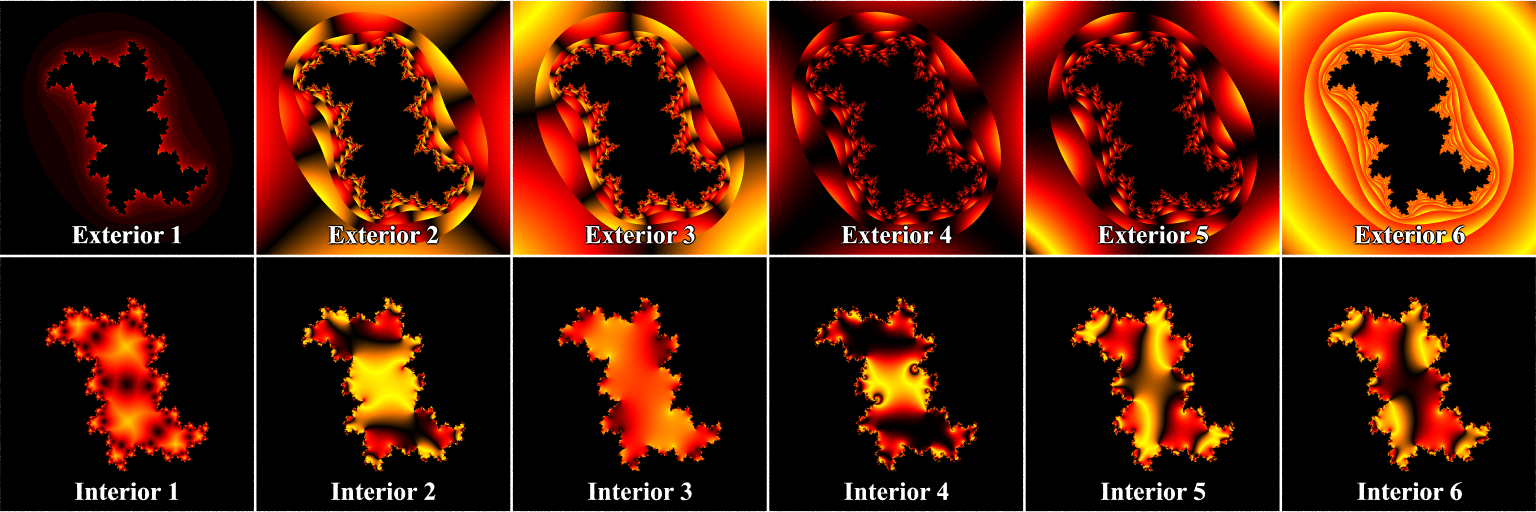
|
|
Different exterior and interior coloring types of fractal patterns |
3.4.7.1.12 Function Pattern
Allows you to use a function { } block as pattern.
pigment {
function { USER_DEFINED_FUNCTIONS }
[PIGMENT_MODIFIERS...]
}
Declaring a function:
By default a function takes three parameters (x,y,z) and you do not have
to explicitly specify the parameter names when declaring it. When using
the identifier, the parameters must be specified.
#declare Foo = function { x + y + z}
pigment {
function { Foo(x, y, z) }
[PIGMENT_MODIFIERS...]
}
On the other hand, if you need more or less than three parameters when declaring a function, you also have to explicitly specify the parameter names.
#declare Foo = function(x,y,z,t) { x + y + z + t}
pigment {
function { Foo(x, y, z, 4) }
[PIGMENT_MODIFIERS...]
}
Using function in a normal:
#declare Foo = function { x + y + z}
normal {
function { Foo(x, y, z) } [Bump_Size]
[MODIFIERS...]
}
3.4.7.1.12.1 What can be used
All float expressions and operators. See the section User-Defined Functions for what is legal in POV-Ray. Of special interest here is the pattern option, that makes it possible to use patterns as functions
#declare FOO = function {
pattern {
checker
}
}
User defined functions (like equations).
Since pigments can be declared as functions, they can also be used in functions. They must be declared first. When using the identifier, you have to specify which component of the color vector should be used. To do this, the dot notation is used: Function(x,y,z).red
#declare FOO = function {pigment { checker } }
pigment {
function { FOO(x,y,z).green }
[PIGMENT_MODIFIERS...]
}
POV-Ray has a large amount of pre-defined functions. These are mainly algebraic surfaces but there is also a mesh function and noise3d function. See section Internal Functions for a complete list and some explanation on the parameters to use. These internal functions can be included through the functions.inc include file.
#include "functions.inc"
#declare FOO = function {pigment { checker } }
pigment {
function { FOO(x,y,z).green & f_noise3d(x*2, y*3,z)}
[PIGMENT_MODIFIERS...]
}
3.4.7.1.12.2 Function Image
Syntax :
function Width, Height { FUNCTION_BODY }
Not a real pattern, but listed here for convenience. This keyword defines a new 'internal' bitmap image type. The pixels of the image are derived from the Function_Body, with Function_Body either being a regular function, a pattern function or a pigment function. In case of a pigment function the output image will be in color, in case of a pattern or regular function the output image will be grayscale. All variants of grayscale pigment functions are available using the regular function syntax, too. In either case the image will use 16 bit per component
Note: Functions are evaluated on the x-y plane. This is different from the pattern image type for the reason that it makes using uv functions easier.
Width and Height specify the resolution of the resulting 'internal' bitmap image.
The image is taken from the square region <0,0,0>, <1,1,0>
The function statement can be used wherever an image specifier
like tga or png may be used. Some uses include
creating heightfields from procedural textures or wrapping a slice of a 3d
texture or function around a cylinder or extrude it along an axis.
Examples:
plane {y, -1
pigment {
image_map {
function 10,10 {
pigment { checker 1,0 scale .5 }
}
}
rotate x*90
}
}
height_field {
function 200,200 {
pattern {
bozo
}
}
translate -0.5
scale 10
pigment {rgb 1}
}
Note: For height fields and other situations where color is not needed
it is easier to use function n,n {pattern{...}} than function n,n {pigment{...}}.
The pattern functions are returning a scalar, not a color vector, thus a pattern is grayscale.
3.4.7.1.13 Gradient Pattern
One of the simplest patterns is the gradient pattern. It is
specified as
pigment {
gradient <Orientation>
[PIGMENT_MODIFIERS...]
}
where <Orientation> is a vector pointing in
the direction that the colors blend. For example
pigment { gradient x } // bands of color vary as you move
// along the "x" direction.
produces a series of smooth bands of color that look like layers of colors
next to each other. Points at x=0 are the first color in the color map. As
the x location increases it smoothly turns to the last color at x=1. Then it
starts over with the first again and gradually turns into the last color at
x=2. In POV-Ray versions older than 3.5 the pattern reverses for negative values of x.
As per POV-Ray 3.5 this is not the case anymore. Using gradient
y or gradient z makes the colors blend along the y- or
z-axis. Any vector may be used but x, y and z are most common.
As a normal pattern, gradient generates a saw-tooth or ramped wave appearance. The syntax is
normal {
gradient <Orientation> [, Bump_Size]
[NORMAL_MODIFIERS...]
}
where the vector <Orientation> is a required
parameter but the float Bump_Size which follows is
optional.
Note: The comma is required especially if Bump_Size is negative.
If only the range -1 to 1 was used of the old gradient, for example in a
sky_sphere, it can be replaced by the planar or marble
pattern and revert the color_map. Also rotate the pattern for other orientations than y.
A more general solution is to use function{abs(x)} as a pattern instead
of gradient x and similar for gradient y and gradient z.
3.4.7.1.14 Granite Pattern
The granite pattern uses a simple 1/f fractal noise function
to give a good granite pattern. This pattern is used with creative color maps
in stones.inc to create some gorgeous layered stone
textures.
As a normal pattern it creates an extremely bumpy surface that looks like a gravel driveway or rough stone.
Note: The appearance of the granite pattern depends on the noise generator used.
The default type is 2. This may be changed using the noise_generator keyword. See the Pattern Modifiers section: noise_generator.
3.4.7.1.15 Leopard Pattern
Leopard creates regular geometric pattern of circular spots. The formula used is: value = Sqr((sin(x)+sin(y)+sin(z))/3)
3.4.7.1.16 Marble Pattern
The marble pattern is very similar to the gradient
x pattern. The gradient pattern uses a default ramp_wave
wave type which means it uses colors from the color map from 0.0 up to 1.0 at
location x=1 but then jumps back to the first color for x > 1 and repeats
the pattern again and again. However the marble pattern uses
the triangle_wave wave type in which it uses the color map from
0 to 1 but then it reverses the map and blends from 1 back to zero. For
example:
pigment {
gradient x
color_map {
[0.0 color Yellow]
[1.0 color Cyan]
}
}
This blends from yellow to cyan and then it abruptly changes back to
yellow and repeats. However replacing gradient x with
marble smoothly blends from yellow to cyan as the x coordinate goes
from 0.0 to 0.5 and then smoothly blends back from cyan to yellow by
x=1.0.
Earlier versions of POV-Ray did not allow you to change wave types. Now that
wave types can be changed for most any pattern, the distinction between
marble and gradient x is only a matter of default
wave types.
When used with turbulence and an appropriate color map, this pattern looks like veins of color of real marble, jade or other types of stone. By default, marble has no turbulence.
The marble pattern has a default color_map built in that results
in a red, black and white pattern with smooth and sharp transitions.
3.4.7.1.17 Onion Pattern
The onion is a pattern of concentric spheres like the layers
of an onion. Value = mod(sqrt(Sqr(X)+Sqr(Y)+Sqr(Z)), 1.0) Each
layer is one unit thick.
3.4.7.1.18 Pavement Pattern
The pavement is a pattern which paves the x-z plane with a single polyform tile. A polyform is a plane figure constructed by joining together identical basic polygons. The number_of_sides is used to choose that basic polygon: an equilateral triangle (3), a square (4) or a hexagon (6). The number_of_tiles is used to choose the number of basic polygons in the tile while pattern is used to choose amongst the variants.
The syntax is:
pigment {
pavement
[PAVEMENT_MODIFIERS...]
}
PAVEMENT_MODIFIERS:
number_of_sides SIDES_VALUE | number_of_tiles TILES_VALUE | pattern PATTERN_VALUE |
exterior EXTERIOR_VALUE | interior INTERIOR_VALUE | form FORM_VALUE |
PATTERN_MODIFIERS
A table of the number of patterns:
| Sides | ||||||
|---|---|---|---|---|---|---|
| 1 | 2 | 3 | 4 | 5 | 6 | |
| 1 | 1 | 1 | 3 | 4 | 12 | |
| 1 | 1 | 2 | 5 | 12 | 35 | |
| 1 | 1 | 3 | 7 | 22 | ||
|
|
The various patterns with 6 squares. |
There is no nomenclature for pattern, they are just numbered from 1 to the maximum relevant value.
form- 0, 1 or 2, a special 3 is allowed for square only which copy the look of
interiorfor some additional variations.
interior- 0, 1 or 2
exterior- 0, 1 or 2; Not used for hexagon.
The form, exterior and interior specify the look of angle used for respectively slow convex (turning side), quick convex (pointy tile) and concave angle (interior angle between many tiles).
- 0 is a normal pointy angle. (a right angle for square)
- 1 is the same as 0, but the pointy angle is broken in two. For square, the two corners are broken so as to share middle angle.
- 2 is a smooth negotiation of the angle, without pointy part.
Note: The case of paving the plane with tiles made of 6 hexagons is not supported because not all such tiles would pave the plane. For example, the ring made of six hexagons is not able to pave the plane.
3.4.7.1.19 Pigment Pattern
Use any pigment as a pattern. Instead of using the pattern directly on the object, a
pigment_pattern converts the pigment to gray-scale first. For each point, the gray-value
is checked against a list and the corresponding item is then used for the texture at
that particular point. For values between listed items, an averaged texture is calculated.
Texture items can be color, pigment, normal or texture and are specified in a
color_map, pigment_map, normal_map or texture_map.
It takes a standard pigment specification.
Syntax:
PIGMENT:
pigment {
pigment_pattern { PIGMENT_BODY }
color_map { COLOR_MAP_BODY } |
colour_map { COLOR_MAP_BODY } |
pigment_map { PIGMENT_MAP_BODY }
}
NORMAL:
normal {
pigment_pattern { PIGMENT_BODY } [Bump_Size]
normal_map { NORMAL_MAP_BODY }
}
TEXTURE:
texture {
pigment_pattern { PIGMENT_BODY }
texture_map { TEXTURE_MAP_BODY }
}
ITEM_MAP_BODY:
ITEM_MAP_IDENTIFIER | ITEM_MAP_ENTRY...
ITEM_MAP_ENTRY:
[ GRAY_VALUE ITEM_MAP_ENTRY... ]
This pattern is also useful when parent and children patterns need to be transformed independently from each other. Transforming the pigment_pattern will not affect the child textures. When any of the child textures should be transformed, apply it to the specific MAP_ENTRY.
This can be used with any pigments, ranging from a simple checker to very complicated nested pigments. For example:
pigment {
pigment_pattern {
checker White, Black
scale 2
turbulence .5
}
pigment_map {
[ 0, checker Red, Green scale .5 ]
[ 1, checker Blue, Yellow scale .2 ]
}
}
Note: This pattern uses a pigment to get the gray values. If you want to get the pattern from an image, you should use the image_pattern.
3.4.7.1.20 Planar Pattern
The planar pattern creates a horizontal stripe plus or minus
one unit above and below the X-Z plane. It is computed by: value =1.0-
min(1, abs(Y)) It starts at 1.0 at the origin and decreases to a minimum
value of 0.0 as the Y values approaches a distance of 1 unit from the X-Z
plane. It remains at 0.0 for all areas beyond that distance. This pattern was
originally created for use with halo or media but
it may be used anywhere any pattern may be used.
3.4.7.1.21 Quilted Pattern
The quilted pattern was originally designed only to be used
as a normal pattern. The quilted pattern is so named because it can create a
pattern somewhat like a quilt or a tiled surface. The squares are actually
3-D cubes that are 1 unit in size.
When used as a normal pattern, this pattern uses a specialized normal
perturbation function. This means that the pattern cannot be used with
normal_map, slope_map or wave type modifiers in a
normal statement.
When used as a pigment pattern or texture pattern, the quilted
pattern is similar to normal quilted but is not identical as are most normals
when compared to pigments.
The two parameters control0 and control1 are used
to adjust the curvature of the seam or gouge area between
the quilts.
The syntax is:
pigment {
quilted
[QUILTED_MODIFIERS...]
}
QUILTED_MODIFIERS:
control0 Value_0 | control1 Value_1 | PIGMENT_MODIFIERS
The values should generally be kept to around the 0.0 to 1.0 range. The default value is 1.0 if none is specified. Think of this gouge between the tiles in cross-section as a sloped line.
|
|
Quilted pattern with c0=0 and different values for c1. |
|
|
Quilted pattern with c0=0.33 and different values for c1. |
|
|
Quilted pattern with c0=0.67 and different values for c1. |
|
|
Quilted pattern with c0=1 and different values for c1. |
This straight slope can be made to curve by adjusting the two control values. The control values adjust the slope at the top and bottom of the curve. A control values of 0 at both ends will give a linear slope, as shown above, yielding a hard edge. A control value of 1 at both ends will give an "s" shaped curve, resulting in a softer, more rounded edge.
The syntax for use as a normal is:
normal {
quilted [Bump_Size]
[QUILTED_MODIFIERS...]
}
QUILTED_MODIFIERS:
control0 Value_0 | control1 Value_1 | PIGMENT_MODIFIERS
3.4.7.1.22 Radial Pattern
The radial pattern is a radial blend that wraps around the
+y-axis. The color for value 0.0 starts at the +x-direction and wraps the
color map around from east to west with 0.25 in the -z-direction, 0.5 in -x,
0.75 at +z and back to 1.0 at +x. Typically the pattern is used with a
frequency modifier to create multiple bands that radiate from the
y-axis. For example:
pigment {
radial
color_map {
[0.5 Black]
[0.5 White]
}
frequency 10
}
creates 10 white bands and 10 black bands radiating from the y axis.
The radial pattern has a default color_map built in that results
in a yellow, magenta and cyan pattern with smooth transitions.
3.4.7.1.23 Ripples Pattern
The ripples pattern was originally designed only to be used
as a normal pattern. It makes the surface look like ripples of water. The
ripples radiate from 10 random locations inside the unit cube area
<0,0,0> to <1,1,1>. Scale the pattern to make the centers closer
or farther apart.
Usually the ripples from any given center are about 1 unit apart. The
frequency keyword changes the spacing between ripples. The
phase keyword can be used to move the ripples outwards for realistic
animation.
The number of ripple centers can be changed with the global parameter
global_settings { number_of_waves Count }
somewhere in the scene. This affects the entire scene. You cannot change the number of wave centers on individual patterns. See the section Number Of Waves for details.
When used as a normal pattern, this pattern uses a specialized normal
perturbation function. This means that the pattern cannot be used with
normal_map, slope_map or wave type modifiers in a normal statement.
When used as a pigment pattern or texture pattern, the ripples
pattern is similar to normal ripples but is not identical as are most normals
when compared to pigments.
3.4.7.1.24 Spherical Pattern
The spherical pattern creates a one unit radius sphere, with its center at
the origin. It is computed by: value = 1.0-min(1, sqrt(X^2 + Y^2 +
Z^2)) It starts at 1.0 at the origin and decreases to a minimum value of 0.0
as it approaches a distance of 1 unit from the origin in any direction. It
remains at 0.0 for all areas beyond that distance. This pattern was
originally created for use with halo or media but
it may be used anywhere any pattern may be used.
3.4.7.1.25 Spiral1 Pattern
The spiral1 pattern creates a spiral that winds around the
z-axis similar to a screw. When viewed sliced in the x-y plane, it looks like
the spiral arms of a galaxy. Its syntax is:
pigment {
spiral1 Number_of_Arms
[PIGMENT_MODIFIERS...]
}
The Number_of_Arms value determines how may arms are
winding around the z-axis.
As a normal pattern, the syntax is
normal {
spiral1 Number_of_Arms [, Bump_Size]
[NORMAL_MODIFIERS...]
}
where the Number_of_Arms value is a required
parameter but the float Bump_Size which follows is
optional.
Note: The comma is required especially if Bump_Size is negative.
The pattern uses the triangle_wave wave type by default but may
use any wave type.
3.4.7.1.26 Spiral2 Pattern
The spiral2 pattern creates a double spiral that winds around
the z-axis similar to spiral1 except that it has two overlapping spirals
which twist in opposite directions. The result sometimes looks like a basket
weave or perhaps the skin of pineapple. The center of a sunflower also has a
similar double spiral pattern. Its syntax is:
pigment {
spiral2 Number_of_Arms
[PIGMENT_MODIFIERS...]
}
The Number_of_Arms value determines how may arms are
winding around the z-axis. As a normal pattern, the syntax is
normal {
spiral2 Number_of_Arms [, Bump_Size]
[NORMAL_MODIFIERS...]
}
where the Number_of_Arms value is a required
parameter but the float Bump_Size which follows is
optional.
Note: The comma is required especially if Bump_Size is negative. The pattern uses the triangle_wave wave type by default but may use any wave type.
3.4.7.1.27 Spotted Pattern
The spotted pattern is identical to the bozo
pattern. Early versions of POV-Ray did not allow turbulence to be used with
spotted. Now that any pattern can use turbulence there is no difference
between bozo and spotted. See the section Bozo for details.
3.4.7.1.28 Tiling Pattern
The tiling pattern creates a series tiles in the x-z plane. See the image below for examples of the twenty-seven available patterns.
The syntax is as follows:
pigment {
tiling Pattern_Number
[PATTERN_MODIFIERS...]
}
 |
The various tiling patterns annotated by tiling pattern and tiling type respectively |
For each pattern, each individual tile of the pattern has the same beveling as the other tiles in that pattern, allowing regular caulking to be defined. For a pattern with N tile types (where N is the tiling type noted in the above image) the main color/texture of the tiles are at x/N with x going from 0 to N-1, and the extreme color/texture caulk for these tiles are at (x+1)/N. The bevel covers the range between these two values.
To begin exploring the tiling pattern right away, see the distribution file ~scenes/textures/pattern/tiling.pov. It uses obvious colors to better illustrate how the feature works, and you can optionally write it's color_map to a text file. Once you get a feel for the break points, you can always define you own map!
3.4.7.1.29 Waves Pattern
The waves pattern was originally designed only to be used as
a normal pattern. It makes the surface look like waves on water. The
waves pattern looks similar to the ripples pattern except
the features are rounder and broader. The effect is to make waves that look
more like deep ocean waves. The waves radiate from 10 random locations inside
the unit cube area <0,0,0> to <1,1,1>. Scale the pattern to make
the centers closer or farther apart.
Usually the waves from any given center are about 1 unit apart. The
frequency keyword changes the spacing between waves. The
phase keyword can be used to move the waves outwards for realistic
animation.
The number of wave centers can be changed with the global parameter
global_settings { number_of_waves Count }
somewhere in the scene. This affects the entire scene. You cannot change the number of wave centers on individual patterns. See the section Number Of Waves for details.
When used as a normal pattern, this pattern uses a specialized normal
perturbation function. This means that the pattern cannot be used with
normal_map, slope_map or wave type modifiers in a normal statement.
When used as a pigment pattern or texture pattern, the waves
pattern is similar to normal waves but is not identical as are most normals
when compared to pigments.
3.4.7.1.30 Wood Pattern
The wood pattern consists of concentric cylinders centered on
the z-axis. When appropriately colored, the bands look like the growth rings
and veins in real wood. Small amounts of turbulence should be added to make
it look more realistic. By default, wood has no turbulence.
Unlike most patterns, the wood pattern uses the
triangle_wave wave type by default. This means that like marble, wood
uses color map values 0.0 to 1.0 then repeats the colors in reverse order
from 1.0 to 0.0. However you may use any wave type.
The wood pattern has a default color_map built in that results
in a light and dark brown pattern with sharp transitions.
3.4.7.1.31 Wrinkles Pattern
The wrinkles pattern was originally designed only to be used
as a normal pattern. It uses a 1/f noise pattern similar to granite but the
features in wrinkles are sharper. The pattern can be used to simulate
wrinkled cellophane or foil. It also makes an excellent stucco texture.
When used as a normal pattern, this pattern uses a specialized normal
perturbation function. This means that the pattern cannot be used with
normal_map, slope_map or wave type modifiers in a
normal statement.
When used as a pigment pattern or texture pattern, the wrinkles
pattern is similar to normal wrinkles but is not identical as are most
normals when compared to pigments.
Note: The appearance of the wrinkles pattern depends on the noise generator used.
The default type is 2. This may be changed using the noise_generator keyword. See the section Pattern Modifiers: noise_generator.
3.4.7.2 Discontinuous Patterns
Some patterns are discontinuous, meaning their slope is infinite. These patterns are not suitable for use as object norms, as objects with discontinuous norms may look odd. These patterns work best for textures and media. They are cells, checker, crackle, hexagon, object, square and triangular.
Note: The cell and crackle patterns are mixed cases, that is, they are discontinuous at their respective boundaries. However, there is no limit to the different number of values, in the range of 0 to 1, that they can generate.
3.4.7.2.1 Cells Pattern
The cells pattern fills 3d space with unit cubes. Each cube gets a
random value from 0 to 1.
cells is not very suitable as a normal as it has no smooth
transitions of one grey value to another.
3.4.7.2.2 Checker Pattern
The checker pattern produces a checkered pattern consisting
of alternating squares of two colors. The syntax is:
pigment { checker [COLOR_1 [, COLOR_2]] [PATTERN_MODIFIERS...] }
If no colors are specified then default blue and green colors are used.
The checker pattern is actually a series of cubes that are one unit in size. Imagine a bunch of 1 inch cubes made from two different colors of modeling clay. Now imagine arranging the cubes in an alternating check pattern and stacking them in layer after layer so that the colors still alternate in every direction. Eventually you would have a larger cube. The pattern of checks on each side is what the POV-Ray checker pattern produces when applied to a box object. Finally imagine cutting away at the cube until it is carved into a smooth sphere or any other shape. This is what the checker pattern would look like on an object of any kind.
You may also use pigment statements in place of the colors. For example:
pigment { checker pigment{Jade}, pigment{Black_Marble} }
This example uses normals:
normal { checker 0.5 }
The float value is an optional bump size. You may also use full normal statements. For example:
normal {
checker normal{gradient x scale .2}, normal{gradient y scale .2}
}
When used with textures, the syntax is
texture { checker texture{T_Wood_3A}, texture{Stone12} }
The checker pattern has a default color_map built in that
results in blue and green tiles.
This use of checker as a texture pattern replaces the special tiles
texture in previous versions of POV-Ray. You may still use
tiles but it may be phased out in future versions so checker textures
are best.
This is a block pattern which cannot use wave types,
color_map, or slope_map modifiers.
3.4.7.2.3 Crackle Pattern
The crackle pattern is a set of random tiled multifaceted cells. The crackle pattern is only semi-procedural, requiring random values to be computed and cached for subsequent queries, with a fixed amount of data per unit-cube in crackle pattern coordinate space. Scaled smaller than the density of actual ray-object-intersections computed, it will eventually lead to a separate crackle cache entry being created for each and every intersection. After the cache reaches a certain size (currently 30mb per thread), new entries for that particular block will be discarded after they are calculated. Starting a new block will allow the caching to resume working again. While discarding the data is of course inefficient, it's still preferable to chewing up 100% of the available physical RAM and then hitting the swap-file.
There is a choice between different types:
Standard Crackle
Mathematically, the set crackle(p)=0 is a 3D Voronoi diagram of a field of semi random points and crackle(p) < 0 is the distance from the set along the shortest path (a Voronoi diagram is the locus of points equidistant from their two nearest neighbors from a set of disjoint points, like the membranes in suds are to the centers of the bubbles).
- With a large scale and no turbulence it makes a pretty good stone wall or floor.
- With a small scale and no turbulence it makes a pretty good crackle ceramic glaze.
- Using high turbulence it makes a good marble that avoids the problem of apparent parallel layers in traditional marble.
Form
pigment {
crackle form <FORM_VECTOR>
[PIGMENT_ITEMS ...]
}
normal {
crackle [Bump_Size]
form <FORM_VECTOR>
[NORMAL_ITEMS ...]
}
Form determines the linear combination of distances used to create the pattern. Form is a vector.
- The first component determines the multiple of the distance to the closest point to be used in determining the value of the pattern at a particular point.
- The second component determines the coefficient applied to the second-closest distance.
- The third component corresponds to the third-closest distance.
The standard form is <-1,1,0> (also the default), corresponding to the difference in the distances to the closest and second-closest points in the cell array. Another commonly-used form is <1,0,0>, corresponding to the distance to the closest point, which produces a pattern that looks roughly like a random collection of intersecting spheres or cells.
- Other forms can create very interesting effects, but it is best to keep the sum of the coefficients low.
- If the final computed value is too low or too high, the resultant pigment will be saturated with the color at the low or high end of the
color_map. In this case, try multiplying the form vector by a constant.
Metric
pigment {
crackle metric METRIC_VALUE
[PIGMENT_ITEMS ...]
}
normal {
crackle [Bump_Size]
metric METRIC_VALUE
[NORMAL_ITEMS ...]
}
Changing the metric changes the function used to determine which cell center is closer, for purposes of determining which cell a particular point falls in. The standard Euclidean distance function has a metric of 2. Changing the metric value changes the boundaries of the cells. A metric value of 3, for example, causes the boundaries to curve, while a very large metric constrains the boundaries to a very small set of possible orientations.
- The default for metric is 2, as used by the standard crackle texture.
- Metrics other than 1 or 2 can lead to substantially longer render times, as the method used to calculate such metrics is not as efficient.
Offset
pigment {
crackle offset OFFSET_VALUE
[PIGMENT_ITEMS ...]
}
normal {
crackle [Bump_Size]
offset OFFSET_VALUE
[NORMAL_ITEMS ...]
}
The offset is used to displace the pattern from the standard xyz space along a fourth dimension.
- It can be used to round off the pointy parts of a cellular normal texture or procedural heightfield by keeping the distances from becoming zero.
- It can also be used to move the calculated values into a specific range if the result is saturated at one end of the color_map.
- The default offset is zero.
Solid
pigment {
crackle solid
[PIGMENT_ITEMS ...]
}
normal {
crackle [Bump_Size]
solid
[NORMAL_ITEMS ...]
}
Causes the same value to be generated for every point within a specific cell. This has practical applications in making easy stained-glass windows or flagstones. There is no provision for mortar, but mortar may be created by layering or texture-mapping a standard crackle texture with a solid one. The default for this parameter is off.
3.4.7.2.4 Hexagon Pattern
The hexagon pattern is a block pattern that generates a
repeating pattern of hexagons in the x-z-plane. In this instance imagine tall
rods that are hexagonal in shape and are parallel to the y-axis and grouped
in bundles like shown in the example image. Three separate colors should be
specified as follows:
pigment {
hexagon [COLOR_1 [, COLOR_2 [, COLOR_3]]]
[PATTERN_MODIFIERS...]
}
|
|
The hexagon pattern. |
The three colors will repeat the hexagonal pattern with hexagon COLOR_1 centered at the origin, COLOR_2 in the +z-direction and COLOR_3 to either side. Each side of the hexagon is one unit long. The hexagonal rods of color extend infinitely in the +y- and -y-directions. If no colors are specified then default blue, green and red colors are used.
You may also use pigment statements in place of the colors. For example:
pigment {
hexagon
pigment { Jade },
pigment { White_Marble },
pigment { Black_Marble }
}
This example uses normals:
normal { hexagon 0.5 }
The float value is an optional bump size. You may also use full normal statements. For example:
normal {
hexagon
normal { gradient x scale .2 },
normal { gradient y scale .2 },
normal { bumps scale .2 }
}
When used with textures, the syntax is...
texture {
hexagon
texture { T_Gold_3A },
texture { T_Wood_3A },
texture { Stone12 }
}
The hexagon pattern has a default color_map built in that results
in red, blue and green tiles.
This is a block pattern which cannot use wave types,
color_map, or slope_map modifiers.
3.4.7.2.5 Object Pattern
The object pattern takes an object as input. It generates a, two item,
color list pattern. Whether a point is assigned to one item or the other depends on
whether it is inside the specified object or not.
Object's used in the object pattern cannot have a texture and must
be solid - these are the same limitations as for bounded_by and
clipped_by.
Syntax:
object {
OBJECT_IDENTIFIER | OBJECT {}
LIST_ITEM_A, LIST_ITEM_B
}
Where OBJ_IDENTIFIER is the target object (which must be declared), or use the full object syntax. LIST_ITEM_A and LIST_ITEM_B are the colors, pigments, or whatever the pattern is controlling. LIST_ITEM_A is used for all points outside the object, and LIST_ITEM_B is used for all points inside the object.
Example:
pigment {
object {
myTextObject
color White
color Red
}
turbulence 0.15
}
Note: This is a block pattern which cannot use wave types, color_map, or slope_map modifiers.
3.4.7.2.6 Square Pattern
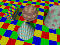
|
The |
|
The square pattern. |
pigment {
square [COLOR_1 [, COLOR_2 [, COLOR_3 [, COLOR_4]]]]
[PATTERN_MODIFIERS...]
}
Each side of the square is one unit long. The square rods of color extend infinitely in the +y and -y directions. If no colors are specified then default blue, green, red and yellow colors are used.
You may also use pigment statements in place of the colors. For example:
pigment {
square
pigment { Aquamarine },
pigment { Turquoise },
pigment { Sienna },
pigment { SkyBlue }
}
When used with textures, the syntax is...
texture {
square
texture{ T_Wood1 },
texture{ T_Wood2 },
texture{ T_Wood4 },
texture{ T_Wood8 }
}
The square pattern has a default color map built in that results in red, blue, yellow and green tiles.
This is a block pattern so, use of wave types, color_map, or slope_map modifiers is not allowed.
3.4.7.2.7 Triangular Pattern
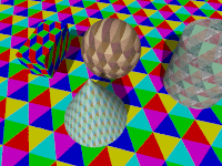
|
The |
|
The triangular pattern. |
pigment {
triangular [COLOR_1 [, COLOR_2 [, COLOR_3 [, COLOR_4 [, COLOR_5 [, COLOR_6]]]]]]
[PATTERN_MODIFIERS...]
}
Each side of the triangle is one unit long. The triangular rods of color extend infinitely in the +y and -y directions. If no colors are specified then default blue, green, red, magenta, cyan and yellow colors are used.
You may also use pigment statements in place of the colors. For example:
pigment {
triangular
pigment { Aquamarine },
pigment { Turquoise },
pigment { Sienna },
pigment { Aquamarine },
pigment { Turquoise },
pigment { SkyBlue }
}
When used with textures, the syntax is...
texture {
triangular
texture{ T_Wood1 },
texture{ T_Wood2 },
texture{ T_Wood4 },
texture{ T_Wood8 },
texture{ T_Wood16 },
texture{ T_Wood10 }
}
The triangular pattern has a default color map built in that results in red, blue, cyan, magenta, yellow and green tiles.
This is a block pattern so, use of wave types, color_map, or slope_map modifiers is not allowed.
3.4.7.3 Normal-Dependent Patterns
Some patterns depend on the normal vector in addition to a position vector. As such, these patterns are suitable for object normals only. They are aoi and slope.
3.4.7.3.1 Aoi Pattern
The aoi pattern can be used with pigment, normal and texture statements. The syntax is as follows:
pigment {
aoi
pigment_map {
[0.0 MyPigmentA]
...
[1.0 MyPigmentZ]
}
}
normal {
aoi
normal_map {
[0.0 MyNormalA]
...
[1.0 MyNormalZ]
}
}
texture {
aoi
texture_map {
[0.0 MyTextureA]
...
[1.0 MyTextureZ]
}
}
It gives a value proportional to the angle between the ray and the surface; for consistency with the slope pattern, values range from 0.5 where ray is tangent to the surface, to 1.0 where perpendicular; in practice, values below 0.5 may occur in conjunction with smooth triangles or meshes.
Note: This differs from the current MegaPOV implementation, where the values range from 0.5 down to 0.0 instead. If compatibility with MegaPOV is desired, it is recommended to mirror the gradient at 0.5, e.g.:
pigment {
aoi
pigment_map {
[0.0 MyPigment3]
[0.2 MyPigment2]
[0.5 MyPigment1]
[0.8 MyPigment2]
[1.0 MyPigment3]
}
}
3.4.7.3.2 Slope Pattern
The slope pattern uses the normal of a surface to calculate the slope
at a given point. It then creates the pattern value dependent on the slope and optionally
the altitude. It can be used for pigments, normals and textures, but not for media densities.For pigments the syntax is:
pigment {
slope {
<Direction> [, Lo_slope, Hi_slope ]
[ altitude <Altitude> [, Lo_alt, Hi_alt ]]
}
[PIGMENT_MODIFIERS...]
}
The slope value at a given point is dependent on the angle between the <Direction> vector and the normal of the surface at that point.
For example:
- When the surface normal points in the opposite direction of the
<Direction>vector (180 degrees), the slope is 0.0. - When the surface normal is perpendicular to the
<Direction>vector (90 degrees), the slope is 0.5. - When the surface normal is parallel to the
<Direction>vector (0 degrees), the slope is 1.0.
When using the simplest variant of the syntax:
slope { <Direction> }
the pattern value for a given point is the same as the slope value. <Direction> is a 3-D vector and will usually be <0,-1,0> for landscapes, but any direction can be used.
By specifying Lo_slope and Hi_slope you get more control:
slope { <Direction>, Lo_slope, Hi_slope }
Lo_slope and Hi_slope specifies which range of slopes are used, so you can control which slope values return which pattern values. Lo_slope is the slope value that returns 0.0 and Hi_slope is the slope value that returns 1.0.
For example, if you have a height_field and <Direction> is set to <0,-1,0>, then the slope values would only range from 0.0 to 0.5 because height_fields cannot have overhangs. If you do not specify Lo_slope and Hi_slope, you should keep in mind that the texture for the flat (horizontal) areas must be set at 0.0 and the texture for the steep (vertical) areas at 0.5 when designing the texture_map. The part from 0.5 up to 1.0 is not used then. But, by setting Lo_slope and Hi_slope to 0.0 and 0.5 respectively, the slope range will be stretched over the entire map, and the texture_map can then be defined from 0.0 to 1.0.
By adding an optional <Altitude> vector:
slope {
<Direction>
altitude <Altitude>
}
the pattern will be influenced not only by the slope but also by a special gradient. <Altitude> is a 3-D vector that specifies the direction of the gradient. When <Altitude> is specified, the pattern value is a weighted average of the slope value and the gradient value. The weights are the lengths of the vectors <Direction> and <Altitude>. So if <Direction> is much longer than <Altitude> it means that the slope has greater effect on the results than the gradient. If on the other hand <Altitude> is longer, it means that the gradient has more effect on the results than the slope.
When adding the <Altitude> vector, the default gradient is defined from 0 to 1 units along the specified axis. This is fine when your object is defined within this range, otherwise a correction is needed. This can be done with the optional Lo_alt and Hi_alt parameters:
slope {
<Direction>
altitude <Altitude>, Lo_alt, Hi_alt
}
They define the range of the gradient along the axis defined by the <Altitude> vector.
For example, with an <Altitude> vector set to y and an object going from -3 to 2 on
the y axis, the Lo_alt and Hi_alt parameters should be set to -3 and 2 respectively.
Note: You should be aware of the following pitfalls when using the slope pattern.
- You may use the turbulence keyword inside slope pattern definitions but it may cause unexpected results. Turbulence is a 3-D distortion of a pattern. Since slope is only defined on surfaces of objects, a 3-D turbulence is not applicable to the slope component. However, if you are using altitude, the altitude component of the pattern will be affected by turbulence.
- If your object is larger than the range of altitude you have specified, you may experience unexpected discontinuities. In that case it is best to adjust the
Lo_altandHi_altvalues so they fit to your object. - The slope pattern does not work for the sky_sphere, because the sky_sphere is a background feature and does not have a surface. similarly, it does not work for media densities.
As of version 3.7 the slope pattern has been extended to specify a reference point instead of a direction; the new syntax variant is as follows:
slope {
point_at <ReferencePoint> [, Lo_Slope, Hi_Slope ]
}
Note: This variant currently does not allow for the altitude keyword to be used.
The functionality is similar to MegaPOV's aoi <ReferencePoint> pattern, except that the values are reversed, i.e. range from 0.0 for surfaces facing away from the point in question, to 1.0 for surfaces facing towards that point; thus, slope { <Vector> } and slope { point_at <Vector>*VeryLargeNumber } have virtually the same effect.
3.4.7.4 Special Patterns
Some patterns are not "real" patterns, but behave like patterns and are used in the same location as a regular pattern. They are average and image.
3.4.7.4.1 Average Pattern
Technically average is not a pattern type but it is listed here
because the syntax is similar to other patterns. Typically a pattern type specifies
how colors or normals are chosen from a pigment_map,
texture_map, density_map, or normal_map
, however average tells POV-Ray to
average together all of the patterns you specify. Average was originally
designed to be used in a normal statement with a normal_map as a
method of specifying more than one normal pattern on the same surface.
However average may be used in a pigment statement with a
pigment_map or in a texture statement with a texture_map
or media density with density_map to average colors too.
When used with pigments, the syntax is:
AVERAGED_PIGMENT:
pigment {
pigment_map {
PIGMENT_MAP_ENTRY...
}
}
PIGMENT_MAP_ENTRY:
[ [Weight] PIGMENT_BODY ]
Where Weight is an optional float value that
defaults to 1.0 if not specified. This weight value is the relative weight
applied to that pigment. Each PIGMENT_BODY is anything which can be
inside a pigment{...} statement. The pigment
keyword and {} braces need not be specified.
Note: The [] brackets are part of the actual
PIGMENT_MAP_ENTRY. They are not notational symbols denoting optional
parts. The brackets surround each entry in the pigment_map.
There may be from 2 to 256 entries in the map.
For example
pigment {
average
pigment_map {
[1.0 Pigment_1]
[2.0 Pigment_2]
[0.5 Pigment_3]
}
}
All three pigments are evaluated. The weight values are multiplied by the
resulting color. They are then divided by the total of the weights which, in
this example is 3.5. When used with texture_map or
density_map it works the same way.
When used with a normal_map in a normal statement, multiple
copies of the original surface normal are created and are perturbed by each
pattern. The perturbed normals are then weighted, added and normalized.
See the sections Pigment Maps and Pigment Lists, Normal Maps and Normal Lists, Texture Maps, and Density Maps and Density Lists for more information.
3.4.7.4.2 Image Pattern
Instead of placing the color of the image on the object like an image_map, an image_pattern specifies an entire texture item (color, pigment, normal or texture) based on the gray value at that point.
This gray-value is checked against a list and the corresponding item is then used for the texture at that particular point. For values between listed items, an averaged texture is calculated.
It takes a standard image specification and has one option, use_alpha, which works similar to use_color or use_index.
Note: See the section Using the Alpha Channel for some important information regarding the use of image_pattern.
Syntax:
PIGMENT:
pigment {
IMAGE_PATTERN
color_map { COLOR_MAP_BODY } |
colour_map { COLOR_MAP_BODY } |
pigment_map { PIGMENT_MAP_BODY }
}
NORMAL:
normal {
IMAGE_PATTERN [Bump_Size]
normal_map { NORMAL_MAP_BODY }
}
TEXTURE:
texture {
IMAGE_PATTERN
texture_map { TEXTURE_MAP_BODY }
}
IMAGE_PATTERN:
image_pattern {
BITMAP_TYPE "bitmap.ext" [gamma GAMMA] [premultiplied BOOL]
[IMAGE_MAP_MODS...]
}
IMAGE_MAP_MOD:
map_type Type | once | interpolate Type | use_alpha
ITEM_MAP_BODY:
ITEM_MAP_IDENTIFIER | ITEM_MAP_ENTRY...
ITEM_MAP_ENTRY:
[ GRAY_VALUE ITEM_MAP_ENTRY... ]
It is also useful for creating texture masks, like the following:
texture {
image_pattern { tga "image.tga" use_alpha }
texture_map {
[0 Mytex ]
[1 pigment { transmit 1 } ]
}
}
Note: This pattern uses an image to get the gray values from. If you want exactly the same possibilities but need to get gray values from a pigment, you can use the pigment_pattern.
While POV-Ray will normally interpret the image pattern input file as a container of linear data irregardless of file type, this can be overridden for any individual image pattern input file by specifying gamma GAMMA immediately after the file name. For example:
image_pattern {
jpeg "foobar.jpg" gamma 1.8
}
This will cause POV-Ray to perform gamma adjustment or -decoding on the input file data before building the image pattern. Alternatively to a numerical value, srgb may be specified to denote that the file format is pre-corrected or encoded using the sRGB transfer function instead of a power-law gamma function. See section Gamma Handling for more information on gamma.
3.4.7.5 Pattern Modifiers
Pattern modifiers are statements or parameters which modify how a pattern is evaluated or tells what to do with the pattern. The complete syntax is:
PATTERN_MODIFIER:
BLEND_MAP_MODIFIER | AGATE_MODIFIER | DENSITY_FILE_MODIFIER |
QUILTED_MODIFIER | BRICK_MODIFIER | SLOPE_MODIFIER |
noise_generator Number| turbulence <Amount> |
octaves Count | omega Amount | lambda Amount |
warp { [WARP_ITEMS...] } | TRANSFORMATION
BLEND_MAP_MODIFIER:
frequency Amount | phase Amount | ramp_wave | triangle_wave |
sine_wave | scallop_wave | cubic_wave | poly_wave [Exponent]
AGATE_MODIFIER:
agate_turb Value
BRICK_MODIFIER:
brick_size Size | mortar Size
DENSITY_FILE_MODIFIER:
interpolate Type
SLOPE_MODIFIERS:
<Altitude>
<Lo_slope,Hi_slope>
<Lo_alt,Hi_alt>
QUILTED_MODIFIER:
control0 Value | control1 Value
PIGMENT_MODIFIER:
PATTERN_MODIFIER | COLOR_LIST | PIGMENT_LIST |
color_map { COLOR_MAP_BODY } | colour_map { COLOR_MAP_BODY } |
pigment_map{ PIGMENT_MAP_BODY } | quick_color COLOR |
quick_colour COLOR
COLOR NORMAL_MODIFIER:
PATTERN_MODIFIER | NORMAL_LIST |
normal_map { NORMAL_MAP_BODY } | slope_map{ SLOPE_MAP_BODY } |
bump_size Amount
TEXTURE_PATTERN_MODIFIER:
PATTERN_MODIFIER | TEXTURE_LIST |
texture_map{ TEXTURE_MAP_BODY }
DENSITY_MODIFIER:
PATTERN_MODIFIER | DENSITY_LIST | COLOR_LIST |
color_map { COLOR_MAP_BODY } | colour_map { COLOR_MAP_BODY } |
density_map { DENSITY_MAP_BODY }
Default values for pattern modifiers:
dist_exp : 0 falloff : 2.0 frequency : 1.0 lambda : 2.0 major_radius : 1 map_type : 0 noise_generator : 2 octaves : 6 omega : 0.5 orientation : <0,0,1> phase : 0.0 poly_wave : 1.0 strength : 1.0 turbulence : <0,0,0>
The modifiers PIGMENT_LIST, quick_color, and pigment_map apply only to pigments. See the section Pigment for details on these pigment-specific pattern modifiers.
The modifiers COLOR_LIST and color_map apply only to pigments and densities. See the sections Pigment and Density for details on these pigment-specific pattern modifiers.
The modifiers NORMAL_LIST, bump_size, slope_map and normal_map apply only to normals. See the section Normal for details on these normal-specific pattern
modifiers.
The TEXTURE_LIST and texture_map modifiers can only be used with patterned textures. See the section Texture Maps for details.
The DENSITY_LIST and density_map modifiers only work with media{density{..}} statements. See the section Density for details.
The agate_turb modifier can only be used with the agate pattern. See the section Agate for details.
The brick_size and mortar modifiers can only be used with the brick pattern. See the section Brick for details.
The control0 and control1 modifiers can only be used with the quilted pattern. See the section Quilted for details.
The interpolate modifier can only be used with the density_file pattern. See the section Density File for details.
The general purpose pattern modifiers in the following sections can be used with pigment, normal, texture, or density patterns.
3.4.7.5.1 Transforming Patterns
The most common pattern modifiers are the transformation modifiers translate, rotate, scale, transform, and matrix. For details on these commands see the section Transformations.
These modifiers may be placed inside pigment, normal, texture, and density statements to change the position, size and orientation of the patterns.
Transformations are performed in the order in which you specify them.
However in general the order of transformations relative to other pattern
modifiers such as turbulence, color_map and other
maps is not important. For example scaling before or after turbulence makes
no difference. The turbulence is done first, then the scaling regardless of
which is specified first. However the order in which transformations are
performed relative to warp statements is important. See the section Warp for details.
3.4.7.5.2 Frequency and Phase
The frequency and phase modifiers act as a type
of scale and translate modifiers for various blend maps. They only have
effect when blend maps are used. Blend maps are color_map,
pigment_map, normal_map, slope_map,
density_map, and texture_map. This discussion uses
a color map as an example but the same principles apply to the other blend
map types.
The frequency keyword adjusts the number of times that a color
map repeats over one cycle of a pattern. For example gradient covers color map values 0 to 1 over the range from x=0 to x=1. By adding frequency 2.0 the color map repeats twice over that same range. The same effect can be achieved using scale 0.5*x so the frequency keyword is not that useful for patterns like gradient.
However the radial pattern wraps the color map around the +y-axis once. If
you wanted two copies of the map (or 3 or 10 or 100) you would have to build
a bigger map. Adding frequency 2.0 causes the color map to be
used twice per revolution. Try this:
pigment {
radial
color_map{
[0.5 color Red]
[0.5 color White]
}
frequency 6
}
The result is six sets of red and white radial stripes evenly spaced around the object.
The float after frequency can be any value. Values greater than
1.0 causes more than one copy of the map to be used. Values from 0.0 to 1.0
cause a fraction of the map to be used. Negative values reverses the map.
The phase value causes the map entries to be shifted so that the map starts and ends at a different place. In the example above if you render successive frames at phase 0 then phase 0.1, phase 0.2, etc. you could create an animation that rotates the stripes. The same effect can be easily achieved by rotating the radial pigment using rotate y*Angle but there are other uses where phase can be handy.
Sometimes you create a great looking gradient or wood color map but you want
the grain slightly adjusted in or out. You could re-order the color map
entries but that is a pain. A phase adjustment will shift everything but
keep the same scale. Try animating a mandel pigment for a color
palette rotation effect.
These values work by applying the following formula
New_Value = fmod ( Old_Value * Frequency + Phase, 1.0 ).
The frequency and phase modifiers have no effect on block patterns checker, brick, and hexagon nor do they effect image_map, bump_map or material_map. They also have no effect in normal statements when used with bumps, dents, quilted or wrinkles because these normal patterns cannot use normal_map or slope_map.
They can be used with normal patterns ripples and waves even though these two patterns cannot use normal_map or slope_map either. When used with ripples or waves, frequency adjusts the space between features and phase can be adjusted from 0.0 to 1.0 to cause the ripples or waves to move relative to their center for animating the features.
3.4.7.5.3 Waveforms
POV-Ray allows you to apply various wave forms to the pattern function
before applying it to a blend map. Blend maps are color_map,
pigment_map, normal_map, slope_map,
density_map, and texture_map.
Most of the patterns which use a blend map, use the entries in the map in
order from 0.0 to 1.0. The effect can most easily be seen when these patterns
are used as normal patterns with no maps. Patterns such as
gradient or onion generate a groove or slot that looks
like a ramp that drops off sharply. This is called a ramp_wave
wave type and it is the default wave type for most patterns. However the
wood and marble patterns use the map from 0.0 to
1.0 and then reverses it and runs it from 1.0 to 0.0. The result is a wave
form which slopes upwards to a peak, then slopes down again in a
triangle_wave. In earlier versions of POV-Ray there was no way to
change the wave types. You could simulate a triangle wave on a ramp wave
pattern by duplicating the map entries in reverse, however there was no way
to use a ramp wave on wood or marble.
Now any pattern that takes a map can have the default wave type overridden. For example:
pigment { wood color_map { MyMap } ramp_wave }
Also available are sine_wave, scallop_wave,
cubic_wave and poly_wave types. These types are of
most use in normal patterns as a type of built-in slope map. The
sine_wave takes the zig-zag of a ramp wave and turns it into a gentle
rolling wave with smooth transitions. The scallop_wave uses the
absolute value of the sine wave which looks like corduroy when scaled small
or like a stack of cylinders when scaled larger. The cubic_wave
is a gentle cubic curve from 0.0 to 1.0 with zero slope at the start and end.
The poly_wave is an exponential function. It is followed by an
optional float value which specifies exponent. For example poly_wave
2 starts low and climbs rapidly at the end while poly_wave
0.5 climbs rapidly at first and levels off at the end. If no float
value is specified, the default is 1.0 which produces a linear function
identical to ramp_wave.
Although any of these wave types can be used for pigments, normals, textures, or density the effect of many of the wave types are not as noticeable on pigments, textures, or density as they are for normals.
Wave type modifiers have no effect on block patterns checker,
brick, object and hexagon nor do they effect
image_map, bump_map or material_map. They
also have no effect in normal statements when used with bumps,
dents, quilted, ripples,
waves, or wrinkles because these normal patterns cannot
use normal_map or slope_map.
3.4.7.5.4 Noise Generators
There are three noise generators implemented. Changing the noise_generator will change
the appearance of noise based patterns, like bozo and granite.
noise_generator 1the noise that was used in POV_Ray 3.1noise_generator 2range corrected version of the old noise, it does not show the plateaus seen withnoise_generator 1noise_generator 3generates Perlin noise
The default is noise_generator 2
Note: The noise_generator can also be set in global_settings
3.4.7.5.5 Warp
The warp statement is a pattern modifier that is similar to
turbulence. Turbulence works by taking the pattern evaluation point and
pushing it about in a series of random steps. However warps push the point in
very well-defined, non-random, geometric ways. The warp
statement also overcomes some limitations of traditional turbulence and
transformations by giving the user more control over the order in which
turbulence, transformation and warp modifiers are applied to the pattern.
The turbulence warp provides an alternative way to specify turbulence. The others modify the pattern in geometric ways.
The syntax for using a warp statement is:
WARP:
warp { WARP_ITEM }
WARP_ITEM:
repeat <Direction> [REPEAT_ITEMS...] |
black_hole <Location>, Radius [BLACK_HOLE_ITEMS...] |
turbulence <Amount> [TURB_ITEMS...]
cylindrical [ orientation VECTOR | dist_exp FLOAT ]
spherical [ orientation VECTOR | dist_exp FLOAT ]
toroidal [ orientation VECTOR | dist_exp FLOAT | major_radius FLOAT ]
planar [ VECTOR , FLOAT ]
REPEAT_ITEMS:
offset <Amount> |
flip <Axis>
BLACK_HOLE_ITEMS:
strength Strength | falloff Amount | inverse |
repeat <Repeat> | turbulence <Amount>
TURB_ITEMS:
octaves Count | omega Amount | lambda Amount
You may have as many separate warp statements as you like in each pattern.
The placement of warp statements relative to other modifiers such as
color_map or turbulence is not important. However
placement of warp statements relative to each other and to transformations is
significant. Multiple warps and transformations are evaluated in the order in
which you specify them. For example if you translate, then warp or warp, then
translate, the results can be different.
3.4.7.5.5.1 Black Hole Warp
A black_hole warp is so named because of its similarity to
real black holes. Just like the real thing, you cannot actually see a black
hole. The only way to detect its presence is by the effect it has on things
that surround it.
Take, for example, a wood grain. Using POV-Ray's normal turbulence and other texture modifier functions, you can get a nice, random appearance to the grain. But in its randomness it is regular - it is regularly random! Adding a black hole allows you to create a localized disturbance in a wood grain in either one or multiple locations. The black hole can have the effect of either sucking the surrounding texture into itself (like the real thing) or pushing it away. In the latter case, applied to a wood grain, it would look to the viewer as if there were a knothole in the wood. In this text we use a wood grain regularly as an example, because it is ideally suitable to explaining black holes. However, black holes may in fact be used with any texture or pattern. The effect that the black hole has on the texture can be specified. By default, it sucks with the strength calculated exponentially (inverse-square). You can change this if you like.
Black holes may be used anywhere a warp is permitted. The syntax is:
BLACK_HOLE_WARP:
warp {
black_hole <Location>, Radius
[BLACK_HOLE_ITEMS...]
}
BLACK_HOLE_ITEMS:
strength Strength | falloff Amount | inverse | type Type |
repeat <Repeat> | turbulence <Amount>
The minimal requirement is the black_hole keyword followed by
a vector <Location> followed by a comma and a
float Radius. Black holes effect all points within the
spherical region around the location and within the radius. This is
optionally followed by any number of other keywords which control how the
texture is warped.
The falloff keyword may be used with a float value to specify
the power by which the effect of the black hole falls off. The default is
two. The force of the black hole at any given point, before applying the
strength modifier, is as follows.
First, convert the distance from the point to the center to a proportion (0 to 1) that the point is from the edge of the black hole. A point on the perimeter of the black hole will be 0.0; a point at the center will be 1.0; a point exactly halfway will be 0.5, and so forth. Mentally you can consider this to be a closeness factor. A closeness of 1.0 is as close as you can get to the center (i.e. at the center), a closeness of 0.0 is as far away as you can get from the center and still be inside the black hole and a closeness of 0.5 means the point is exactly halfway between the two.
Call this value c. Raise c to the power specified in falloff.
By default Falloff is 2, so this is c^2 or c squared. The resulting value is
the force of the black hole at that exact location and is used, after
applying the strength scaling factor as described below, to
determine how much the point is perturbed in space. For example, if c is 0.5
the force is 0.5^2 or 0.25. If c is 0.25 the force is 0.125. But if c is
exactly 1.0 the force is 1.0. Recall that as c gets smaller the point is
farther from the center of the black hole. Using the default power of 2, you
can see that as c reduces, the force reduces exponentially in an
inverse-square relationship. Put in plain English, it means that the force is
much stronger (by a power of two) towards the center than it is at the
outside.
By increasing falloff, you can increase the magnitude of the
falloff. A large value will mean points towards the perimeter will hardly be
affected at all and points towards the center will be affected strongly. A
value of 1.0 for falloff will mean that the effect is linear. A
point that is exactly halfway to the center of the black hole will be
affected by a force of exactly 0.5. A value of falloff of less
than one but greater than zero means that as you get closer to the outside,
the force increases rather than decreases. This can have some uses but there
is a side effect. Recall that the effect of a black hole ceases outside its
perimeter. This means that points just within the perimeter will be affected
strongly and those just outside not at all. This would lead to a visible
border, shaped as a sphere. A value for falloff of 0 would mean
that the force would be 1.0 for all points within the black hole, since any
number larger 0 raised to the power of 0 is 1.0.
The strength keyword may be specified with a float value to
give you a bit more control over how much a point is perturbed by the black
hole. Basically, the force of the black hole (as determined above) is
multiplied by the value of strength, which defaults to 1.0. If
you set strength to 0.5, for example, all points within the black hole will
be moved by only half as much as they would have been. If you set it to 2.0
they will be moved twice as much.
There is a rider to the latter example, though - the movement is clipped to
a maximum of the original distance from the center. That is to say, a point
that is 0.75 units from the center may only be moved by a maximum of 0.75
units either towards the center or away from it, regardless of the value of
strength. The result of this clipping is that you will have an
exclusion area near the center of the black hole where all points whose final
force value exceeded or equaled 1.0 were moved by a fixed amount.
If the inverse keyword is specified then the points
pushed away from the center instead of being pulled in.
The repeat keyword followed by a vector, allows you to simulate
the effect of many black holes without having to explicitly declare them.
Repeat is a vector that tells POV-Ray to use this black hole at multiple
locations. Using repeat logically divides your scene up into
cubes, the first being located at <0,0,0> and going to
<Repeat>. Suppose your repeat vector was <1,5,2>. The
first cube would be from <0,0,0> to < 1,5,2>. This cube repeats,
so there would be one at < -1,-5,-2>, <1,5,2>, <2,10,4> and
so forth in all directions, ad infinitum.
When you use repeat, the center of the black hole does not
specify an absolute location in your scene but an offset into each block. It
is only possible to use positive offsets. Negative values will produce
undefined results.
Suppose your center was <0.5,1,0.25> and the repeat vector is <2,2,2>. This gives us a block at < 0,0,0> and <2,2,2>, etc. The centers of the black hole's for these blocks would be <0,0,0> + < 0.5,1.0,0.25>, i. e. <0.5,1.0,0.25>, and < 2,2,2> + <0.5,1.0,0.25>, i. e. < 2,5,3.0,2.25>.
Due to the way repeats are calculated internally, there is a restriction on the values you specify for the repeat vector. Basically, each black hole must be totally enclosed within each block (or cube), with no part crossing into a neighboring one. This means that, for each of the x, y and z dimensions, the offset of the center may not be less than the radius, and the repeat value for that dimension must be >=the center plus the radius since any other values would allow the black hole to cross a boundary. Put another way, for each of x, y and z
Radius <= Offset or Center <= Repeat - Radius.
If the repeat vector in any dimension is too small to fit this criteria, it will be increased and a warning message issued. If the center is less than the radius it will also be moved but no message will be issued.
Note that none of the above should be read to mean that you cannot
overlap black holes. You most certainly can and in fact this can produce some
most useful effects. The restriction only applies to elements of the
same black hole which is repeating. You can declare a second black
hole that also repeats and its elements can quite happily overlap the first
and causing the appropriate interactions. It is legal for the repeat value
for any dimension to be 0, meaning that POV-Ray will not repeat the black
hole in that direction.
The turbulence can only be used in a black hole with
repeat. It allows an element of randomness to be inserted into the way
the black holes repeat, to cause a more natural look. A good example would be
an array of knotholes in wood - it would look rather artificial if each
knothole were an exact distance from the previous.
The turbulence vector is a measurement that is added to each
individual black hole in an array, after each axis of the vector is multiplied
by a different random amount ranging from 0 to 1. The resulting actual
position of the black hole's center for that particular repeat element is
random (but consistent, so renders will be repeatable) and somewhere within
the above coordinates. There is a rider on the use of turbulence, which
basically is the same as that of the repeat vector. You cannot specify a
value which would cause a black hole to potentially cross outside of its
particular block.
In summary: For each of x, y and z the offset of the center must be >=radius and the value of the repeat must be >= center + radius + turbulence. The exception being that repeat may be 0 for any dimension, which means do not repeat in that direction.
Some examples are given by
warp {
black_hole <0, 0, 0>, 0.5
}
warp {
black_hole <0.15, 0.125, 0>, 0.5
falloff 7
strength 1.0
repeat <1.25, 1.25, 0>
turbulence <0.25, 0.25, 0>
inverse
}
warp {
black_hole <0, 0, 0>, 1.0
falloff 2
strength 2
inverse
}
3.4.7.5.5.2 Repeat Warp
The repeat warp causes a section of the pattern to be
repeated over and over. It takes a slice out of the pattern and makes
multiple copies of it side-by-side. The warp has many uses but was originally
designed to make it easy to model wood veneer textures. Veneer is made by
taking very thin slices from a log and placing them side-by-side on some
other backing material. You see side-by-side nearly identical ring patterns
but each will be a slice perhaps 1/32th of an inch deeper.
The syntax for a repeat warp is
REPEAT_WARP:
warp { repeat <Direction> [REPEAT_ITEMS...] }
REPEAT_ITEMS:
offset <Amount> | flip <Axis>
The repeat vector specifies the direction in which the
pattern repeats and the width of the repeated area. This vector must lie
entirely along an axis. In other words, two of its three components must be
0. For example
pigment {
wood
warp { repeat 2*x }
}
which means that from x=0 to x=2 you get whatever the pattern usually is.
But from x=2 to x=4 you get the same thing exactly shifted two units over in
the x-direction. To evaluate it you simply take the x-coordinate modulo 2.
Unfortunately you get exact duplicates which is not very realistic. The
optional offset vector tells how much to translate the pattern
each time it repeats. For example
pigment {
wood
warp {repeat x*2 offset z*0.05}
}
means that we slice the first copy from x=0 to x=2 at z=0 but at x=2 to x=4 we offset to z=0.05. In the 4 to 6 interval we slice at z=0.10. At the n-th copy we slice at 0.05 n z. Thus each copy is slightly different. There are no restrictions on the offset vector.
Finally the flip vector causes the pattern to be flipped or
mirrored every other copy of the pattern. The first copy of the pattern in
the positive direction from the axis is not flipped. The next farther is, the
next is not, etc. The flip vector is a three component x, y, z vector but
each component is treated as a boolean value that tells if you should or
should not flip along a given axis. For example
pigment {
wood
warp {repeat 2*x flip <1,1,0>}
}
means that every other copy of the pattern will be mirrored about the x- and y- axis but not the z-axis. A non-zero value means flip and zero means do not flip about that axis. The magnitude of the values in the flip vector does not matter.
3.4.7.5.5.3 Turbulence Warp
Inside the warp statement, the keyword turbulence followed by a float or vector may be
used to stir up any pigment, normal or density. A number of
optional parameters may be used with turbulence to control how it is
computed. The syntax is:
TURBULENCE_ITEM: turbulence <Amount> | octaves Count | omega Amount | lambda Amount
Typical turbulence values range from the default 0.0, which is no turbulence, to 1.0 or more, which is very turbulent. If a vector is specified different amounts of turbulence are applied in the x-, y- and z-direction. For example
turbulence <1.0, 0.6, 0.1>
has much turbulence in the x-direction, a moderate amount in the y-direction and a small amount in the z-direction.
Turbulence uses a random noise function called DNoise. This is
similar to the noise used in the bozo pattern except that
instead of giving a single value it gives a direction. You can think of it as
the direction that the wind is blowing at that spot. Points close together
generate almost the same value but points far apart are randomly
different.
Turbulence uses DNoise to push a point around in several steps
called octaves. We locate the point we want to evaluate, then
push it around a bit using turbulence to get to a different point then look
up the color or pattern of the new point.
It says in effect Do not give me the color at this spot... take a few random steps in different directions and give me that color. Each step is typically half as long as the one before. For example:
|
The magnitude of these steps is controlled by the turbulence value. There are three additional parameters which control how turbulence is computed. They are |
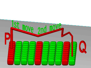
|
|
Turbulence random walk. |
3.4.7.5.5.4 Octaves
The octaves keyword may be followed by an integer value to
control the number of steps of turbulence that are computed. Legal values
range from 1 to <10. The default value of 6 is a fairly high value; you
will not see much change by setting it to a higher value because the extra
steps are too small. Float values are truncated to integer. Smaller numbers
of octaves give a gentler, wavy turbulence and computes faster. Higher
octaves create more jagged or fuzzy turbulence and takes longer to
compute.
3.4.7.5.5.5 Lambda
The lambda parameter controls how statistically different the
random move of an octave is compared to its previous octave. The default
value is 2.0 which is quite random. Values close to lambda 1.0 will
straighten out the randomness of the path in the diagram above. The zig-zag
steps in the calculation are in nearly the same direction. Higher values can
look more swirly under some circumstances.
3.4.7.5.5.6 Omega
The omega value controls how large each successive octave
step is compared to the previous value. Each successive octave of turbulence
is multiplied by the omega value. The default omega 0.5 means
that each octave is 1/2 the size of the previous one. Higher omega values
mean that 2nd, 3rd, 4th and up octaves contribute more turbulence giving a
sharper, crinkly look while smaller omegas give a fuzzy kind of
turbulence that gets blurry in places.
3.4.7.5.5.7 Mapping using warps
With the cylindrical, spherical and toroidal warps you can wrap checkers,
bricks and other patterns around cylinders, spheres, tori and other objects. In essence, these
warps use the same mapping as the image maps use.
The syntax is as follows:
CYLINDRICAL_WARP:
warp { cylindrical [CYLINDRICAL_ITEMS...]}
CYLINDRICAL_ITEMS:
orientation VECTOR | dist_exp FLOAT
SPHERICAL_WARP:
warp { spherical [SPHERICAL_ITEMS...]}
SPHERICAL_ITEMS:
orientation VECTOR | dist_exp FLOAT
TOROIDAL_WARP:
warp { toroidal [TOROIDAL_ITEMS...]}
TOROIDAL_ITEMS:
orientation VECTOR | dist_exp FLOAT | major_radius FLOAT
PLANAR_WARP:
warp { planar [ VECTOR , FLOAT ]}
CUBIC_WARP:
warp { cubic }
These defaults are in affect:
orientation <0,0,1> dist_exp 0 major_radius 1
Although these warps do 3D mapping, some concession had to be made on depth.
The distance exponent is controlled by using the dist_exp keyword. When using the default value of 0, imagine a box from <0,0> to <1,1> stretching to infinity along the orientation vector.
The distance keyword is evaluated as follows:
sphere: distance from origincylinder: distance from y-axistorus: distance from major radius
The planar warp was made to make a pattern act like an image_map, of infinite size and can be useful in combination with other mapping-warps. By default the pigment in the XY-plane is extruded along
the Z-axis. The pigment can be taken from an other plane, by specifying the optional vector (normal of the plane) and float (distance along the normal). The result, again, is extruded along the Z-axis.
The cubic warp requires no parameters, and maps an area in the x-y plane between <0,0> and <1,1> around the origin in the same way as uv-mapping an origin-centered cube-shaped box would. The cubic warp works with any object whereas the uv-mapping only works for the box object. See the section on box uv-mapping for details.
The following code examples produced the images below:
torus {
1, 0.5
pigment {
hexagon
scale 0.1
warp {
toroidal
orientation y
dist_exp 1
major_radius 1
}
}
}
sphere {
0,1
pigment {
hexagon
scale <0.5/pi,0.25/pi,1>*0.1
warp {
spherical
orientation y
dist_exp 1
}
}
}
cylinder {
-y, y, 1
pigment {
hexagon
scale <0.5/pi, 1, 1>*0.1
warp {
cylindrical
orientation y
dist_exp 1
}
}
}
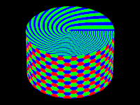
|
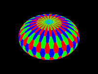
|
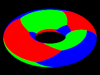
|
|
cylindrical warp |
spherical warp |
toroidal warp |
3.4.7.5.5.8 Turbulence versus Turbulence Warp
The POV-Ray language contains an ambiguity and limitation on the way you
specify turbulence and transformations such as
translate, rotate, scale,
matrix, and transform transforms. Usually the turbulence
is done first. Then all translate, rotate, scale, matrix, and transform
operations are always done after turbulence regardless of the order in which
you specify them. For example this
pigment {
wood
scale .5
turbulence .2
}
works exactly the same as
pigment {
wood
turbulence .2
scale .5
}
The turbulence is always first. A better example of this limitation is with uneven turbulence and rotations.
pigment {
wood
turbulence 0.5*y
rotate z*60
}
// as compared to
pigment {
wood
rotate z*60
turbulence 0.5*y
}
The results will be the same either way even though you would think it should look different.
We cannot change this basic behavior in POV-Ray now because lots of scenes would potentially render differently if suddenly the order transformation vs. turbulence mattered when in the past, it did not.
However, by specifying our turbulence inside warp statement you tell POV-Ray that the order in which turbulence, transformations and other warps are applied is significant. Here is an example of a turbulence warp.
warp { turbulence <0,1,1> octaves 3 lambda 1.5 omega 0.3 }
The significance is that this
pigment {
wood
translate <1,2,3> rotate x*45 scale 2
warp { turbulence <0,1,1> octaves 3 lambda 1.5 omega 0.3 }
}
produces different results than this...
pigment {
wood
warp { turbulence <0,1,1> octaves 3 lambda 1.5 omega 0.3 }
translate <1,2,3> rotate x*45 scale 2
}
You may specify turbulence without using a warp statement. However you cannot control the order in which they are evaluated unless you put them in a warp.
The evaluation rules are as follows:
- First any turbulence not inside a warp statement is applied regardless of the order in which it appears relative to warps or transformations.
- Next each warp statement, translate, rotate, scale or matrix one-by-one, is applied in the order the user specifies. If you want turbulence done in a specific order, you simply specify it inside a warp in the proper place.
3.4.7.5.5.9 Turbulence
The turbulence pattern modifier is still supported for compatibility
issues, but it is better nowadays to use the warp turbulence feature,
which does not have turbulence's limitation in transformation order
(turbulence is always applied first, before any scale, translate or
rotate, whatever the order you specify). For a detailed discussion see
Turbulence versus Turbulence Warp
The old-style turbulence is handled slightly differently when used with the agate, marble, spiral1, spiral2, and wood textures.
3.4.7.6 Image Map
When all else fails and none of the pigment pattern types meets your needs you can use an image_map to wrap a 2-D bit-mapped image around your 3-D objects.
3.4.7.6.1 Specifying an Image Map
The syntax for an image_map is:
IMAGE_MAP:
pigment {
image_map {
[BITMAP_TYPE] "bitmap[.ext]" [gamma GAMMA] [premultiplied BOOL]
[IMAGE_MAP_MODS...]
}
[PIGMENT_MODFIERS...]
}
IMAGE_MAP:
pigment {
image_map {
FUNCTION_IMAGE
}
[PIGMENT_MODFIERS...]
}
BITMAP_TYPE:
exr | gif | hdr | iff | jpeg | pgm | png | ppm | sys | tga | tiff
IMAGE_MAP_MODS:
map_type Type | once | interpolate Type |
filter Palette, Amount | filter all Amount |
transmit Palette, Amount | transmit all Amount
FUNCTION_IMAGE:
function I_WIDTH, I_HEIGHT { FUNCTION_IMAGE_BODY }
FUNCTION_IMAGE_BODY:
PIGMENT | FN_FLOAT | pattern { PATTERN [PATTERN_MODIFIERS] }
After the optional BITMAP_TYPE keyword is a string expression containing the name of a bitmapped image file of the specified type. If the BITMAP_TYPE is not given, the same type is expected as the type set for output.
For example:
plane { -z,0
pigment {
image_map {png "Eggs.png"}
}
}
plane { -z,0
pigment {
image_map {"Eggs"}
}
}
The second method will look for, and use "Eggs.png" if the output file type is set to be png (Output_File_Type=N in INI-file or +FN on command line). It is particularly useful when the image used in the image_map is also rendered with POV-Ray.
Several optional modifiers may follow the file specification. The modifiers are described below.
Note: Earlier versions of POV-Ray allowed some modifiers before the BITMAP_TYPE but that syntax is being phased out in favor of the syntax described here.
Note: The sys format is a system-specific format. See the Output File Type section for more information.
Filenames specified in the image_map statements will be searched for in the home (current) directory first and, if not found, will then be searched for in directories specified by any +L or Library_Path options active. This would facilitate keeping all your image maps files in a separate subdirectory and giving a Library_Path option to specify where your library of image maps are. See Library Paths for details.
By default, the image is mapped onto the x-y-plane. The image is projected onto the object as though there were a slide projector somewhere in the -z-direction. The image exactly fills the square area from (x,y) coordinates (0,0) to (1,1) regardless of the image's original size in pixels. If you would like to change this default you may translate, rotate or scale the pigment or texture to map it onto the object's surface as desired.
In the section Checker, the checker pigment pattern is explained. The checks are described as solid cubes of colored clay from which objects are carved. With image maps you should imagine that each pixel is a long, thin, square, colored rod that extends parallel to the z-axis. The image is made from rows and columns of these rods bundled together and the object is then carved from the bundle.
If you would like to change this default orientation you may translate, rotate or scale the pigment or texture to map it onto the object's surface as desired.
The file name is optionally followed by one or more BITMAP_MODIFIERS. The filter, filter all, transmit, and transmit all modifiers are specific to image maps and are discussed in the following sections. An image_map may also use generic bitmap modifiers map_type,
once and interpolate described in Bitmap Modifiers
3.4.7.6.2 The Gamma Option
The default gamma handling rules for any image input file can be overridden by specifying gamma GAMMA immediately after the file name. For example:
image_map {
jpeg "foobar.jpg" gamma 1.8
interpolate 2
}
Alternatively to a numerical value, srgb may be specified to denote that the file is encoded or pre-corrected using the sRGB transfer function instead of a power-law gamma function.
See section Gamma Handling for more information on gamma.
3.4.7.6.3 The Filter and Transmit Bitmap Modifiers
To make all or part of an image map transparent you can specify filter and/or transmit values for the color palette/registers of PNG, GIF or IFF pictures (at least for the modes that use palettes). You can do this by adding the keyword filter or transmit following the filename. The keyword is followed by two numbers. The first number is the palette number value and the second is the amount of transparency. The values should be separated by a comma. For
example:
image_map {
gif "mypic.gif"
filter 0, 0.5 // Make color 0 50% filtered transparent
filter 5, 1.0 // Make color 5 100% filtered transparent
transmit 8, 0.3 // Make color 8 30% non-filtered transparent
}
You can give the entire image a filter or transmit value using filter all Amount or transmit all Amount. For example:
image_map {
gif "stnglass.gif"
filter all 0.9
}
Note: Early versions of POV-Ray used the keyword alpha to specify filtered transparency however that word is often used to describe non-filtered transparency. For this reason alpha is no longer
used.
See the section Color Expressions for details on the differences between filtered and non-filtered transparency.
3.4.7.6.4 Using the Alpha Channel
Another way to specify non-filtered transmit transparency in an image map is by using the alpha channel. POV-Ray will automatically use the alpha channel for transmittance when one is stored in the image. PNG file format allows you to store a different transparency for each color index in the PNG file, if desired. If your paint programs support this feature of PNG you can do the transparency editing within your paint program rather than specifying transmit values for each color in the POV file. Since PNG and TGA image formats can also store full alpha channel (transparency) information you can generate image maps that have transparency which is not dependent on the color of a pixel but rather its location in the image.
Although POV uses transmit 0.0 to specify no transparency and 1.0 to specify full transparency, the alpha data ranges from 0 to 255 in the opposite direction. Alpha data 0 means the same as transmit 1.0 and alpha data 255 produces transmit 0.0.
Note: In version 3.7 alpha handling for image file output has changed. Effectively, the background now requires a filter or transmit value in order for alpha transparency to work properly.
Previous versions of POV-Ray always expected straight alpha for file input, this has been changed on a per-file-format basis as follows:
- PNG will use straight alpha as per specification.
- OpenEXR and TIFF will use associated alpha as per specifications.
- TGA and BMP 32-bit RGBA will use straight alpha, retaining file input compatibility for now, until a final decision has been made on these formats.
Additionally the premultiplied parameter may be used to specify the input image alpha handling. This boolean parameter specifies whether the file is stored in premultiplied associated or non-premultiplied straight alpha format, overriding the file format specific default. This keyword has no effect on files without an alpha channel. Like the gamma, it MUST immediately follow the filename, though the order does not matter.
Note: The following mechanism has some limitations with colored highlights.
When generating non-premultiplied alpha output to a classic low-dynamic-range file format (e.g. PNG), transparency of particularly bright areas will now be reduced, in order to better preserve highlights on transparent objects.
Note: When using an input image in a material_map, bump_map, or image_pattern definition, the following conditions apply.
- For material maps, no alpha premultiplication handling is done whatsoever, instead the data as stored in the file is used.
- For bump maps and image patterns, images with an alpha channel are treated as if they had a black background, unless the alpha channel itself is used.
Note: See also background and sky_sphere for additional information.
Activating alpha output via Output_Alpha=on or +UA, when used with unsupported file formats generates a warning.
3.4.7.7 Bitmap Modifiers
A bitmap modifier is a modifier used inside an image_map,
bump_map or material_map to specify how the 2-D
bitmap is to be applied to the 3-D surface. Several bitmap modifiers apply to
specific kinds of maps and they are covered in the appropriate sections. The
bitmap modifiers discussed in the following sections are applicable to all
three types of bitmaps.
3.4.7.7.1 The once Option
Normally there are an infinite number of repeating image maps, bump maps
or material maps created over every unit square of the x-y-plane like tiles.
By adding the once keyword after a file name you can eliminate
all other copies of the map except the one at (0,0) to (1,1). In image maps,
areas outside this unit square are treated as fully transparent. In bump
maps, areas outside this unit square are left flat with no normal
modification. In material maps, areas outside this unit square are textured
with the first texture of the texture list.
For example:
image_map {
gif "mypic.gif"
once
}
3.4.7.7.2 The map_type Option
The default projection of the image onto the x-y-plane is called a
planar map type. This option may be changed by adding the
map_type keyword followed by an integer number specifying the way to
wrap the image around the object.
A map_type 0 gives the default planar mapping already
described.
A map_type 1 gives a spherical mapping. It assumes that the
object is a sphere of any size sitting at the origin. The y-axis is the
north/south pole of the spherical mapping. The top and bottom edges of the
image just touch the pole regardless of any scaling. The left edge of the
image begins at the positive x-axis and wraps the image around the sphere
from west to east in a -y-rotation. The image covers the sphere exactly once.
The once keyword has no meaning for this mapping type.
With map_type 2 you get a cylindrical mapping. It assumes that
a cylinder of any diameter lies along the y-axis. The image wraps around the
cylinder just like the spherical map but the image remains one unit tall from
y=0 to y=1. This band of color is repeated at all heights unless the
once keyword is applied.
Finally map_type 5 is a torus or donut shaped mapping. It
assumes that a torus of major radius one sits at the origin in the x-z-plane.
The image is wrapped around similar to spherical or cylindrical maps. However
the top and bottom edges of the map wrap over and under the torus where they
meet each other on the inner rim.
Types 3 and 4 are still under development.
Note: The map_type option may also be applied to
bump_map and material_map statements.
For example:
sphere{<0,0,0>,1
pigment{
image_map {
gif "world.gif"
map_type 1
}
}
}
3.4.7.7.3 The interpolate Option
Adding the interpolate keyword can smooth the jagged look of a bitmap. When POV-Ray checks a color for an image map or a bump amount for a bump map, it often checks a point that is not directly on top of one pixel but sort of between several differently colored pixels. Interpolations return an in-between value so that the steps between the pixels in the map will look smoother.
Although interpolate is legal in material maps, the color index is interpolated before the texture is chosen. It does not interpolate the final color as you might hope it would. In general, interpolation of material maps serves no useful purpose but this may be fixed in future versions.
There are currently three types of interpolation: interpolate 2 gives bilinear interpolation, interpolate 3 gives bicubic, and interpolate 4 gives normalized distance.
For example:
image_map {
gif "mypic.gif"
interpolate 2
}
The default is no interpolation. Normalized distance is the slowest, bilinear does a better job of picking the between color, and arguably, bicubic interpolation is a slight improvement, however it is subject to over-sharpening at some color borders. Normally bilinear is used.
If your map looks jagged, try using interpolation instead of going to a higher resolution image. The results can be very good.
3.4.8 Media
The media statement is used to specify particulate matter suspended in a medium such air or water. It can be used to specify smoke, haze, fog, gas, fire, dust etc. Previous versions of POV-Ray had two incompatible systems for generating such effects. One was halo for effects enclosed in a transparent or semi-transparent object. The other was atmosphere for effects that permeate the entire scene. This duplication of systems was complex and unnecessary. Both halo
and atmosphere have been eliminated. See Why are Interior and Media Necessary? for further details on this change. See Object Media
for details on how to use media with objects. See Atmospheric Media for details on using media for atmospheric effects outside of objects. This section and the sub-sections which follow explains the details of the various media options which are useful for either object media or atmospheric media.
Media works by sampling the density of particles at some specified number of points along the ray's path. Sub-samples are also taken until the results reach a specified confidence level. POV-Ray provides three methods of sampling. When used in an object's interior statement, sampling only occurs inside the object. When used for atmospheric media, the samples run from
the camera location until the ray strikes an object. Therefore for localized effects, it is best to use an enclosing object even though the density pattern might only produce results in a small area whether the media was enclosed or not.
The complete syntax for a media statement is as follows:
MEDIA:
media { [MEDIA_IDENTIFIER] [MEDIA_ITEMS...] }
MEDIA_ITEMS:
method Number | intervals Number | samples Min, Max |
confidence Value | variance Value | ratio Value | jitter Value
absorption COLOR | emission COLOR | aa_threshold Value |
aa_level Value |
scattering {
Type, COLOR [ eccentricity Value ] [ extinction Value ]
} |
density {
[DENSITY_IDENTIFIER] [PATTERN_TYPE] [DENSITY_MODIFIER...]
} |
TRANSFORMATIONS
DENSITY_MODIFIER:
PATTERN_MODIFIER | DENSITY_LIST | COLOR_LIST |
color_map { COLOR_MAP_BODY } | colour_map { COLOR_MAP_BODY } |
density_map { DENSITY_MAP_BODY }
Media default values:
aa_level : 3 aa_threshold : 0.1 absorption : <0,0,0> confidence : 0.9 emission : <0,0,0> intervals : 1 jitter : 0.0 method : 3 ratio : 0.9 samples : Min 1, Max 1 variance : 1/128 SCATTERING COLOR : <0,0,0> eccentricity : 0.0 extinction : 1.0
If a media identifier is specified, it must be the first item. All other media items may be specified in any order. All are optional. You may have multiple density statements in a single media statement. See Multiple Density vs. Multiple Media for details. Transformations apply only to the density statements which have been already specified. Any density after a transformation is not affected. If the media has no density statements and none was specified in any media identifier, then the transformation has no effect. All other media items except for density and transformations override default values or any previously set values for this media statement.
Note: Some media effects depend upon light sources. However the participation of a light source depends upon the media_interaction and media_attenuation keywords. See Atmospheric Media Interaction and Atmospheric Attenuation for details.
Note: If you specify transmit or filter to create a transparent container object, absorption media will always cast a shadow. The same applies to scattering media unless extinction is set to zero, so if a shadow is not desired, use the no_shadow keyword for the container object. This does not apply to emission media as it never casts a shadow.
3.4.8.2 Media Types
There are three types of particle interaction in media: absorbing, emitting, and scattering. All three activities may occur in a single media. Each of these three specifications requires a color. Only the red, green, and blue components of the color are used. The filter and transmit values are ignored. For this reason it is permissible to use one float value to specify an intensity of white color. For example, the following two lines are legal and produce the same results:
emission 0.75 emission rgb <0.75,0.75,0.75>
3.4.8.2.1 Absorption
The absorption keyword specifies a color of light which is absorbed when looking through the media. For example, absorption rgb<0,1,0> blocks the green light but permits red and blue to get through. Therefore a white object behind the media will appear magenta. The default value is rgb<0,0,0> which means no light is absorbed, meaning all light passes through normally.
3.4.8.2.2 Emission
The emission keyword specifies the color of the light emitted from the particles. Particles which emit light are visible without requiring additional illumination. However, they will only illuminate other objects if radiosity is used with media on. This is similar to an object with high ambient values. The default value is rgb<0,0,0> which means no light is emitted.
3.4.8.2.3 Scattering
The syntax of a scattering statement is:
SCATTERING:
scattering {
Type, COLOR [ eccentricity Value ] [ extinction Value ]
}
The first float value specifies the type of scattering. This is followed by the color of the scattered light. The default value if no scattering statement is given is rgb <0,0,0> which means no scattering occurs.
The scattering effect is only visible when light is shining on the media from a light source. This is similar to diffuse reflection off of an object. In addition to reflecting light, scattering media also absorbs light like an absorption media. The balance between how much absorption occurs for a given amount of scattering is controlled by the optional extinction keyword and a single float value. The default value of 1.0 gives an extinction effect that matches the scattering. Values such as extinction 0.25 give 25% the normal amount. Using extinction 0.0 turns it off completely. Any value other than the 1.0 default is contrary to the real physical model but decreasing extinction can give you more artistic flexibility.
The integer value Type specifies one of five different scattering phase functions representing the different models: isotropic, Mie (haze and murky atmosphere), Rayleigh, and Henyey-Greenstein.
Type 1, isotropic scattering is the simplest form of scattering because it is independent of direction. The amount of light scattered by particles in the atmosphere does not depend on the angle between the viewing direction and the incoming light.
Types 2 and 3 are Mie haze and Mie murky scattering which are used for relatively small particles such as minuscule water droplets of fog, cloud particles, and particles responsible for the polluted sky. In this model the scattering is extremely directional in the forward direction, i.e. the amount of scattered light is largest when the incident light is anti-parallel to the viewing direction (the light goes directly to the viewer). It is smallest when the incident light is parallel to the viewing direction. The haze and murky atmosphere models differ in their scattering characteristics. The murky model is much more directional than the haze model.
 |
|
The Mie haze scattering function |
 |
|
The Mie murky scattering function |
Type 4 Rayleigh scattering models the scattering for extremely small particles such as molecules of the air. The amount of scattered light depends on the incident light angle. It is largest when the incident light is parallel or anti-parallel to the viewing direction and smallest when the incident light is perpendicular to the viewing direction. You should note that the Rayleigh model used in POV-Ray does not take the dependency of scattering on the wavelength into account.
 |
|
The Rayleigh scattering function |
Type 5 is the Henyey-Greenstein scattering model. It is based on an analytical function and can be used to model a large variety of different scattering types. The function models an ellipse with a given eccentricity e. This eccentricity is specified by the optional keyword eccentricity which is only used for scattering type five. The default eccentricity value of zero defines isotropic scattering while positive values lead to scattering in the direction of the light and negative values lead to scattering in the opposite direction of the light. Larger values of e (or smaller values in the negative case) increase the directional property of the scattering.
 |
|
The Henyey-Greenstein scattering function for different eccentricity values |
Note: See the section on Light Groups for additional information when using scattering media in a light group.
3.4.8.3 Sampling Parameters & Methods
Media effects are calculated by sampling the media along the path of the ray. It uses a process called Monte Carlo integration. POV-Ray provides three different types of media sampling. The method keyword lets you specify what sampling type is used.
Note: As of version 3.5 the default sampling method is 3, and it's default for intervals is 1. Sampling methods 1 and 2 have been retained for legacy purposes.
Sample method 3 uses adaptive sampling (similar to adaptive anti-aliasing) which is very much like the sampling method used in POV-Ray 3.0 atmosphere. This code was written from the ground-up to work with media. However, adaptive sampling works by taking another sample between two existing samples if there is too much variance in the original two samples. This leads to fewer samples being taken in areas where the effect from the media remains constant. The adaptive sampling is only performed if the minimum samples are set to 3 or more.
You can specify the anti-aliasing recursion depth using the aa_level keyword followed by an integer. You can specify the anti-aliasing threshold by using the aa_threshold followed by a float. The default for aa_level is 4 and the default aa_threshold is 0.1. jitter also works with method 3.
Note: It is usually best to only use one interval with method 3. Too many intervals can lead to artifacts, and POV will create more intervals if it needs them.
Sample method 1 used the intervals keyword to specify the integer number of intervals used to sample the ray. For object media, the intervals are spread between the entry and exit points as the ray passes through the container object. For atmospheric media, the intervals spans the entire length of the ray from its start until it hits an object. For media types which interact with spotlights or cylinder lights, the intervals which are not illuminated by these light types are weighted differently than the illuminated intervals when distributing samples.
The ratio keyword distributes intervals differently between lit and unlit areas. The default value of ratio 0.9 means that lit intervals get more samples than unlit intervals. Note that the total number of intervals must exceed the number of illuminated intervals. If a ray passes in and out of 8 spotlights but you have only specified 5 intervals then an error occurs.
The samples Min, Max keyword specifies the minimum and maximum number of samples taken per interval. The default values are samples 1,1. The value for Max may be omitted, in which case the range Min = Max will be used.
As each interval is sampled, the variance is computed. If the variance is below a threshold value, then no more samples are needed. The variance and confidence keywords specify the permitted variance allowed and the confidence that you are within that variance. The exact calculations are quite complex and involve chi-squared tests and other statistical principles too messy to describe here. The default values are variance 1.0/128 and confidence
0.9. For slower more accurate results, decrease the variance and increase the confidence.
Note: The maximum number of samples limits the calculations even if the proper variance and confidence are never reached.
Sample method 2 distributed samples evenly along the viewing ray or light ray. The latter can make things look smoother sometimes. If you specify a maximum number of samples higher than the minimum number of samples, POV will take additional samples, but they will be random, just like in method 1. Therefore, it is suggested you set the max samples equal to the minimum samples.
jitter will cause method 2 to look similar to method 1. It should be followed by a float, and a value of 1 will stagger the samples in the full range between samples.
3.4.8.4 Density
Particles of media are normally distributed in constant density throughout the media. However, the density statement allows you to vary the density across space using any of POV-Ray's pattern functions such as those used in textures. If no density statement is given then the density remains a constant value of 1.0 throughout the media. More than one density may be specified per media statement. See Multiple Density vs. Multiple Media.
The syntax for density is:
DENSITY:
density {
[DENSITY_IDENTIFIER]
[DENSITY_TYPE]
[DENSITY_MODIFIER...]
}
DENSITY_TYPE:
PATTERN_TYPE | COLOR
DENSITY_MODIFIER:
PATTERN_MODIFIER | DENSITY_LIST | color_map { COLOR_MAP_BODY } |
colour_map { COLOR_MAP_BODY } | density_map { DENSITY_MAP_BODY }
The density statement may begin with an optional density identifier. All subsequent values modify the defaults or the values in the identifier. The next item is a pattern type. This is any one of POV-Ray's pattern functions such as bozo, wood, gradient, waves, etc. Of particular usefulness are the spherical, planar, cylindrical, and boxed patterns which were previously available only for use with our discontinued halo feature. All patterns return a value from 0.0 to 1.0. This value is interpreted as the density of the media at that particular point. See the section Pattern for details on particular pattern types. Although a solid COLOR pattern is legal, in general it is used only when the density statement is inside a density_map.
3.4.8.4.1 General Density Modifiers
A density statement may be modified by any of the general pattern modifiers such as transformations, turbulence and warp. See Pattern Modifiers for details. In addition, there are several density-specific modifiers which can be used.
3.4.8.4.2 Density with color_map
Typically, a media uses just one constant color throughout. Even if you vary the density, it is usually just one color which is specified by the absorption, emission, or scattering keywords. However, when using emission to simulate fire or explosions, the center of the flame (high density area) is typically brighter and white or yellow. The outer edge of the flame (less density) fades to orange, red, or in some cases deep blue. To model the density-dependent change in color which is visible, you may specify a color_map. The pattern function returns a value from 0.0 to 1.0 and the value is passed to the color map to compute what color or blend of colors is used. See Color Maps for details on how pattern values work with color_map. This resulting color is multiplied by the absorption, emission and scattering color. Currently there is no way to specify different color maps for each media type within the same media statement.
Consider this example:
media {
emission 0.75
scattering {1, 0.5}
density {
spherical
color_map {
[0.0 rgb <0,0,0.5>]
[0.5 rgb <0.8, 0.8, 0.4>]
[1.0 rgb <1,1,1>]
}
}
}
The color map ranges from white at density 1.0 to bright yellow at density 0.5 to deep blue at density 0. Assume we sample a point at density 0.5. The emission is 0.75*<0.8,0.8,0.4> or <0.6,0.6,0.3>. Similarly the scattering color is 0.5*<0.8,0.8,0.4> or <0.4,0.4,0.2>.
For block pattern types checker, hexagon, and brick you may specify a color list such as this:
density {
checker
density {rgb<1,0,0>}
density {rgb<0,0,0>}
}
See Color List Pigments which describes how pigment uses a color list. The same principles apply when using them with density.
3.4.8.4.3 Density Maps and Density Lists
In addition to specifying blended colors with a color map you may create a blend of densities using a density_map. The syntax for a density map is identical to a color map except you specify a density in each map entry (and not a color).
The syntax for density_map is as follows:
DENSITY_MAP:
density_map { DENSITY_MAP_BODY }
DENSITY_MAP_BODY:
DENSITY_MAP_IDENTIFIER | DENSITY_MAP_ENTRY...
DENSITY_MAP_ENTRY:
[ Value DENSITY_BODY ]
Where Value is a float value between 0.0 and 1.0 inclusive and each DENSITY_BODY is anything which can be inside a density{...} statement. The density keyword and {} braces need not be specified.
Note: The [] brackets are part of the actual DENSITY_MAP_ENTRY. They are not notational symbols denoting optional parts. The brackets surround each entry in the density map.
There may be from 2 to 256 entries in the map.
Density maps may be nested to any level of complexity you desire. The densities in a map may have color maps or density maps or any type of density you want.
Density lists may also be used with block patterns such as checker, hexagon and brick, as well as the object pattern object.
For example:
density {
checker
density { Flame scale .8 }
density { Fire scale .5 }
}
Note: In the case of block patterns the density wrapping is required around the density information.
A density map is also used with the average density type. See Average for details.
You may declare and use density map identifiers but the only way to declare a density block pattern list is to declare a density identifier for the entire density.
3.4.8.4.4 Multiple Density vs. Multiple Media
It is possible to have more than one media specified per object and it is legal to have more than one density per media. The effects are quite different.
Consider this example:
object {
MyObject
pigment { rgbf 1 }
interior {
media {
density { Some_Density }
density { Another_Density }
}
}
}
As the media is sampled, calculations are performed for each density pattern at each sample point. The resulting samples are multiplied together. Suppose one density returned rgb<.8,.8,.4> and the other returned rgb<.25,.25,0>. The resulting color is rgb<.2,.2,0>.
Note: In areas where one density returns zero, it will wipe out the other density. The end result is that only density areas which overlap will be visible. This is similar to a CSG intersection operation. Now consider:
object {
MyObject
pigment { rgbf 1 }
interior {
media {
density { Some_Density }
}
media {
density { Another_Density }
}
}
}
In this case each media is computed independently. The resulting colors are added together. Suppose one density and media returned rgb<.8,.8,.4> and the other returned rgb<.25,.25,0>. The resulting color is rgb<1.05,1.05,.4>. The end result is that density areas which overlap will be especially bright and all areas will be visible. This is similar to a CSG union operation. See the sample scene ~scenes\interior\media\media4.pov for an example which illustrates this.
3.4.8.1 Interior
Introduced in POV-Ray 3.1 is an object modifier statement called
interior. The syntax is:
INTERIOR:
interior { [INTERIOR_IDENTIFIER] [INTERIOR_ITEMS...] }
INTERIOR_ITEM:
ior Value | caustics Value | dispersion Value |
dispersion_samples Samples | fade_distance Distance |
fade_power Power | fade_color <Color>
MEDIA...
Interior default values:
ior : 1.0 caustics : 0.0 dispersion : 1.0 dispersion_samples : 7 fade_distance : 0.0 fade_power : 0.0 fade_color : <0,0,0>
The interior contains items which describe the properties of the interior of the object. This is in contrast to the texture and interior_texture which describe the surface properties only. The interior of an object is only of interest if it has a transparent texture which allows you to see inside the object. It also applies only to solid objects which have a well-defined inside/outside distinction.
Note: The open keyword, or clipped_by modifier also allows you to see inside but interior features may not render properly. They should be avoided if accurate interiors are required.
Interior identifiers may be declared to make scene files more readable and to parameterize scenes so that changing a single declaration changes many values. An identifier is declared as follows.
INTERIOR_DECLARATION: #declare IDENTIFIER = INTERIOR | #local IDENTIFIER = INTERIOR
Where IDENTIFIER is the name of the identifier up to 40 characters long and INTERIOR is any valid interior statement. See #declare vs. #local for information on identifier scope.
3.4.8.1.1 Why are Interior and Media Necessary?
In previous versions of POV-Ray, most of the items in the interior statement were previously part of the finish statement. Also the halo statement which was once part of the texture statement has been discontinued and has been replaced by the media statement which is part of interior.
You are probably asking WHY? As explained earlier, the interior contains items which describe the properties of the interior of the object. This is in contrast to the texture which describes the surface properties only. However this is not just a philosophical change. There were serious inconsistencies in the old model.
The main problem arises when a texture_map or other patterned texture is used. These features allow you to create
textures that are a blend of two textures and which vary the entire texture from one point to another. It does its blending by fully evaluating the apparent color as though only one texture was applied and then fully reevaluating it with the other texture. The two final results are blended.
It is totally illogical to have a ray enter an object with one index or refraction and then recalculate with another index. The result is not an average of the two ior values. Similarly it makes no sense to have a ray enter at one ior and exit at a different ior without transitioning between them along the way. POV-Ray only calculates refraction as the ray enters or leaves. It cannot incrementally compute a changing ior through the interior of an object. Real world objects such as optical fibers or no-line bifocal eyeglasses can have variable iors but POV-Ray cannot simulate them.
Similarly the halo calculations were not performed as the
syntax implied. Using a halo in such multi-textured objects did
not vary the halo through the interior of the object. Rather,
it computed two separate halos through the whole object and averaged the
results. The new design for media which replaces
halo makes it possible to have media that varies throughout the
interior of the object according to a pattern but it does so independently of
the surface texture. Because there are other changes in the design of this
feature which make it significantly different, it was not only moved to the
interior but the name was changed.
During our development, someone asked if we will create patterned interiors
or a hypothetical interior_map feature. We will not. That would
defeat the whole purpose of moving these features in the first place. They
cannot be patterned and have logical or self-consistent results.
3.4.8.1.2 Empty and Solid Objects
It is very important that you know the basic concept behind empty and solid objects in POV-Ray to fully understand how features like interior and translucency are used. Objects in POV-Ray can either be solid, empty or filled with (small) particles.
A solid object is made from the material specified by its pigment and finish statements (and to some degree its normal statement). By default all objects are assumed to be solid. If you assign a stone texture to a sphere you will get a ball made completely of stone. It is like you had cut this ball from a block of stone. A glass ball is a massive sphere made of glass. You should be aware that solid objects are conceptual things. If you clip away parts of the sphere you will clearly see that the interior is empty and it just has a very thin surface.
This is not contrary to the concept of a solid object used in POV-Ray. It is
assumed that all space inside the sphere is covered by the sphere's
interior. Light passing through the object is affected by
attenuation and refraction properties. However there is no room for any other
particles like those used by fog or interior media.
Empty objects are created by adding the hollow keyword (see
Hollow) to the object statement. An empty (or hollow) object is
assumed to be made of a very thin surface which is of the material specified
by the pigment, finish and normal statements. The object's interior is
empty, it normally contains air molecules.
An empty object can be filled with particles by adding fog or atmospheric media to the scene or by adding an interior media to the object. It is very important to understand that in order to fill an object with any kind of particles it first has to be made hollow.
There is a pitfall in the empty/solid object implementation that you have to be aware of.
In order to be able to put solid objects inside a media or fog, a test has to be made for every ray that passes through the media. If this ray travels through a solid object the media will not be calculated. This is what anyone will expect. A solid glass sphere in a fog bank does not contain fog.
The problem arises when the camera ray is inside any non-hollow object. In this case the ray is already traveling through a solid object and even if the media's container object is hit and it is hollow, the media will not be calculated. There is no way of telling between these two cases.
POV-Ray has to determine whether the camera is inside any object prior to tracing a camera ray in order to be able to correctly render medias when the camera is inside the container object. There is no way around doing this.
The solution to this problem (that will often happen with infinite objects like planes) is to make those objects hollow too. Thus the ray will travel through a hollow object, will hit the container object and the media will be calculated.
3.4.8.1.3 Scaling objects with an interior
All the statements that can be put in an interior represent aspects of the matter that an object is made of. Scaling an object, changing its size, does not change its matter. Two pieces of the same quality steel, one twice as big as the other, both have the same density. The bigger piece is quite a bit heavier though.
So, in POV-Ray, if you design a lens from a glass with an ior of 1.5
and you scale it bigger, the focal distance of the lens will get longer
as the ior stays the same. For light attenuation it means that an object will be
darker after being scaled up. The light intensity decreases a certain
amount per pov-unit. The object has become bigger, more pov-units, so more light is faded.
The fade_distance, fade_power themselves have not been changed.
The same applies to media. Imagine media as a density of particles,
you specify 100 particles per cubic pov-unit. If we scale a 1 cubic
pov-unit object to be twice as big in every direction, we will have a
total of 800 particles in the object. The object will look different,
as we have more particles to look through. Yet the objects density is
still 100 particles per cubic pov-unit. In media this particle
density is set by the color after emission, absorption, or in
the scattering statement
#version 3.5;
global_settings {
assumed_gamma 1.0
}
camera {location <0, 0,-12.0> look_at 0 angle 30 }
#declare Container_T =
texture {
pigment {rgbt <1,1,1,1>}
finish {ambient 0 diffuse 0}
}
#declare Scale=2;
box { //The reference
<-1,-1,0>,<1,1,.3>
hollow
texture {Container_T}
interior {
media {
intervals 1
samples 1,1
emission 1
}
}
translate <-2.1,0,0>
}
box { //Object scaled twice as big
<-1,-1,0>,<1,1,.3> //looks different but same
hollow //particle density
texture {Container_T}
interior {
media {
intervals 1
samples 1,1
emission 1
}
}
scale Scale
translate<0,0,12>
}
box { //Object scaled twice as big
<-1,-1,0>,<1,1,.3> //looks the same but particle
hollow //density scaled down
texture {Container_T}
interior {
media {
intervals 1
samples 1,1
emission 1/Scale
}
}
scale Scale
translate<0,0,12>
translate<4.2,0,0>
}
The third object in the scene above, shows what to do, if you want to scale the object and want it to keep the same look as before. The interior feature has to be divided by the same amount, that the object was scaled by. This is only possible when the object is scaled uniform.
In general, the correct approach is to scale the media density proportionally to the change in container volume. For non-uniform scaling to get an unambiguous result, that can be explained in physical terms, we need to do:
Density*sqrt(3)/vlength(Scale)
where Density is your original media density and Scale is the scaling vector applied to the container.
Note: The density modifiers inside the density{}
statement are scaled along with the object.
3.4.8.1.4 Refraction
When light passes through a surface either into or out of a dense medium
the path of the ray of light is bent. Such bending is called
refraction. The amount of bending or refracting of light depends upon
the density of the material. Air, water, crystal and diamonds all have
different densities and thus refract differently. The index of
refraction or ior value is used by scientists to describe the
relative density of substances. The ior keyword is used in
POV-Ray in the interior to turn on refraction and to specify the
ior value. For example:
object { MyObject pigment {Clear } interior { ior 1.5 } }
The default ior value of 1.0 will give no refraction. The index of refraction for air is 1.0, water is 1.33, glass is 1.5 and diamond is 2.4.
Normally transparent or semi-transparent surfaces in POV-Ray do not refract
light. Earlier versions of POV-Ray required you to use the
refraction keyword in the finish statement to turn on
refraction. This is no longer necessary. Any non-zero ior value
now turns refraction on.
In addition to turning refraction on or off, the old refraction
keyword was followed by a float value from 0.0 to 1.0. Values in between 0.0
and 1.0 would darken the refracted light in ways that do not correspond to
any physical property. Many POV-Ray scenes were created with intermediate
refraction values before this bug was discovered so the feature has been
maintained. A more appropriate way to reduce the brightness of refracted
light is to change the filter or
transmit value in the colors
specified in the pigment statement or to use the fade_power
and fade_distance keywords.
See Attenuation.
Note: Neither the ior nor refraction keywords cause the
object to be transparent. Transparency only occurs if there is a non-zero
filter or transmit value in the color.
The refraction and ior keywords were originally
specified in finish but are now properly specified in
interior. They are accepted in finish
for backward compatibility and generate a warning message.
3.4.8.1.5 Dispersion
For all materials with a ior different from 1.0 the refractive index is not constant throughout the spectrum. It changes as a function of wavelength. Generally the refractive index decreases as the wavelength increases. Therefore light passing through a material will be separated according to wavelength. This is known as chromatic dispersion.
By default POV-Ray does not calculate dispersion as light travels through a
transparent object. In order to get a more realistic effect the dispersion
and dispersion_samples keywords can be added to the
interior{} block. They will simulate dispersion by creating a
prismatic color effect in the object.
The dispersion value is the ratio of refractive indices for violet to
red. It controls the strength of dispersion (how much the colors are spread out) used.
A DISPERSION_VALUE of 1 will give no dispersion, good values are 1.01 to 1.1.
Note: There will be no dispersion, unless the ior keyword has
been specified in interior{ }. An ior of 1 is legal. The ior has no
influence on the dispersion strength, only on the angle of refraction.
As POV-Ray does not use wavelengths for raytracing, a spectrum is simulated.
The dispersion_samples value controls the amount of color-steps and
smoothness in the spectrum. The default value is 7, the minimum is 2. Values up to
100 or higher may be needed to get a very smooth result.
3.4.8.1.5.1 Dispersion & Caustics
Dispersion only affects the interior of an object and has no effect on faked
caustics (See Faked Caustics).
To see the effects of dispersion in caustics, photon mapping is needed. See the sections
Photons and Photons and Dispersion.
3.4.8.1.6 Attenuation
Light attenuation is used to model the decrease in light intensity as
the light travels through a transparent object. The keywords fade_power, fade_distance and fade_color are specified in the interior statement.
The fade_distance value determines the distance the light has to travel to reach half intensity while the fade_power value determines how fast the light will fall off. fade_color colorizes the attenuation. For realistic effects a fade power of 1 to 2 should be used. Default values for fade_power and fade_distance is 0.0 which turns this feature off. Default for fade_color is <0,0,0>, if fade_color is <1,1,1> there is no attenuation. The actual colors give colored attenuation. <1,0,0> looks red, not cyan as in media.
The attenuation is calculated by a formula similar to that used for light source attenuation.
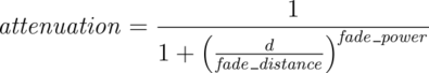
|
|
Media Attenuation |
If you set fade_power in the interior of an object at 1000 or above, a realistic exponential attenuation function will be used:
Attenuation = exp(-depth/fade_dist)
The fade_power and fade_distance keywords were
originally specified in finish but are now properly specified in
interior. They are accepted in finish for backward
compatibility and generate a warning message.
3.4.8.1.7 Simulated Caustics
Caustics are light effects that occur if light is reflected or refracted by specular reflective or refractive surfaces. Imagine a glass of water standing on a table. If sunlight falls onto the glass you will see spots of light on the table. Some of the spots are caused by light being reflected by the glass while some of them are caused by light being refracted by the water in the glass.
Since it is a very difficult and time-consuming process to actually calculate those effects (though it is not impossible), see the sections Photons. POV-Ray uses a quite simple method to simulate caustics caused by refraction. The method calculates the angle between the incoming light ray and the surface normal. Where they are nearly parallel it makes the shadow brighter. Where the angle is greater, the effect is diminished. Unlike real-world caustics, the effect does not vary based on distance. This caustic effect is limited to areas that are shaded by the transparent object. You will get no caustic effects from reflective surfaces nor in parts that are not shaded by the object.
The caustics Power keyword controls the
effect. Values typically range from 0.0 to 1.0 or higher. Zero is the default
which is no caustics. Low, non-zero values give broad hot-spots while higher
values give tighter, smaller simulated focal points.
The caustics keyword was originally specified in
finish but is now properly specified in interior. It is
accepted in finish for backward compatibility and generates a
warning message.
3.4.8.1.8 Object-Media
The interior statement may contain one or more media
statements. Media is used to simulate suspended particles such as smoke,
haze, or dust. Or visible gasses such as steam or fire and explosions. When
used with an object interior, the effect is constrained by the object's
shape. The calculations begin when the ray enters an object and ends when
it leaves the object. This section only discusses media when used with
object interior. The complete syntax and an explanation of all of the
parameters and options for media is given in the section
Media.
Typically the object itself is given a fully transparent texture however media also works in partially transparent objects. The texture pattern itself does not effect the interior media except perhaps to create shadows on it. The texture pattern of an object applies only to the surface shell. Any interior media patterns are totally independent of the texture.
In previous versions of POV-Ray, this feature was called halo
and was part of the texture specification along with
pigment, normal, and finish. See the section: Why are Interior and Media Necessary? for an explanation of the reasons for the change.
Media may also be specified outside an object to simulate atmospheric media. There is no constraining object in this case. If you only want media effects in a particular area, you should use object media rather than only relying upon the media pattern. In general it will be faster and more accurate because it only calculates inside the constraining object. See Atmospheric Media for details on unconstrained uses of media.
You may specify more than one media statement per
interior statement. In that case, all of the media participate and
where they overlap, they add together.
Any object which is supposed to have media effects inside it, whether those
effects are object media or atmospheric media, must have the hollow on
keyword applied. Otherwise the media is blocked. See the section: Empty and Solid Objects
for details.
3.4.9 Include Files
This section covers the include files that come with every distribution of POV-Ray. File location varies, so see your platform specific documentation for more information.
3.4.9.1 Main Files
The main include files in alphabetical order:
3.4.9.1.1 Arrays.inc
This file contains macros for manipulating arrays.
ARRAYS_WriteDF3(Array, FileName, BitDepth): Write an array to a df3 file.
Parameters:
Array= The array that contains the data.FileName= The name of the file to be written.BitDepth= The size of the binary word.
Note: See the #write directive for more information.
Rand_Array_Item(Array, Stream): Randomly Picks an item from a 1D array.
Parameters:
Array= The array from which to choose the item.Stream= A random number stream.
Resize_Array(Array, NewSize): Resize a 1D array, retaining its contents.
Parameters:
Array= The array to be resized.NewSize= The desired new size of the array.
Reverse_Array(Array): Reverses the order of items in a 1D array.
Parameters:
Array= The array to be reversed.
Sort_Compare(Array, IdxA, IdxB): This macro is used by the Sort_Array()
and Sort_Partial_Array() macros. The given macro works for 1D arrays of floats, but
you can redefine it in your scene file for more complex situations, arrays of vectors or
multidimensional arrays for example. Just make sure your macro returns true if the item at IdxA <
the item at IdxB, and otherwise returns false.
Parameters:
Array= The array containing the data being sorted.IdxA, IdxB= The array offsets of the data elements being compared.
Sort_Swap_Data(Array, IdxA, IdxB): This macro is used by the Sort_Array()
and Sort_Partial_Array() macros. The given macro works for 1D arrays only,
but you can redefine it in your scene file to handle multidimensional arrays if needed.
The only requirement is that your macro swaps the data at IdxA with that at IdxB.
Parameters:
Array= The array containing the data being sorted.IdxA, IdxB= The array offsets of the data elements being swapped.
Sort_Array(Array): This macro sorts a 1D array of floats, though you can
redefine the Sort_Compare() and Sort_Swap_Data() macros to
handle multidimensional arrays and other data types.
Parameters:
Array= The array to be sorted.
Sort_Partial_Array(Array, FirstInd, LastInd): This macro is like
Sort_Array(), but sorts a specific range of an array instead of the whole array.
Parameters:
Array= The array to be sorted.FirstInd, LastInd= The start and end indices of the range being sorted.
3.4.9.1.2 Chars.inc
This file includes 26 upper-case letter and other characters defined as objects. The size of all characters is 4 * 5 * 1. The center of the bottom side of a character face is set to the origin, so you may need to translate a character appropriately before rotating it about the x or z axes.
Letters:
char_A, char_B, char_C,
char_D, char_E, char_F,
char_G, char_H, char_I,
char_J, char_K, char_L,
char_M, char_N, char_O,
char_P, char_Q, char_R,
char_S, char_T, char_U,
char_V, char_W, char_X,
char_Y, char_Z
Numerals:
char_0, char_1,
char_2, char_3,
char_4, char_5,
char_6, char_7,
char_8, char_9
Symbols:
char_Dash, char_Plus, char_ExclPt,
char_Amps, char_Num, char_Dol,
char_Perc, char_Astr, char_Hat,
char_LPar, char_RPar, char_AtSign,
char_LSqu, char_RSqu
Usage:
#include "chars.inc"
.
.
object {char_A ...}
3.4.9.1.3 Colors.inc
This file is mainly a list of predefined colors, but also has a few color manipulation macros.
3.4.9.1.3.1 Predefined colors
This file contains 127 predefined colors that you can use in your scenes. Simply #include them in your scene file to use them:
#include "colors.inc"
These basic colors:
- Red
- Green
- Blue
- Yellow
- Cyan
- Magenta
- Clear
- White
- Black
A series of percentage grays that are useful for fine-tuning lighting color values and for other areas where subtle variations of grays are needed, and a palette 99 additional color definitions are available. See the distribution file ~include/colors.inc for more details.
3.4.9.1.3.2 Color macros
In POV-Ray all colors are handled in RGB color space with a component for the amount of red, green and blue light. However, not everybody thinks this is the most intuitive way to specify colors. For your convenience there are macros included in colors.inc that converts between a few different types of color spaces.
The three supported color spaces:
RGB= < Red, Green, Blue, Filter, Transmit >HSL= < Hue, Saturation, Lightness, Filter, Transmit >HSV= < Hue, Saturation, Value, Filter, Transmit >
Note: The Hue parameter is given in degrees.
CHSL2RGB(Color): Converts a color given in HSL space to one in RGB space.
Parameters:
Color=HSLcolor to be converted.
CRGB2HSL(Color): Converts a color given in RGB space to one in HSL space.
Parameters:
Color=RGBcolor to be converted.
CHSV2RGB(Color): Converts a color given in HSV space to one in RGB space.
Parameters:
Color=HSVcolor to be converted.
CRGB2HSV(Color): Converts a color given in RGB space to one in HSV space.
Parameters:
Color=RGBcolor to be converted.
Convert_Color(SourceType, DestType, Color): Converts a color from one color space to another. Color spaces available are: RGB, HSL, and HSV:
Parameters:
SourceType= Color space of input color.DestType= Desired output color space.Color= Color to be converted, in SourceType color space.
3.4.9.1.4 Consts.inc
This file defines a number of constants, including things such as mapping types and ior definitions.
3.4.9.1.4.1 Vector constants
o= < 0, 0, 0> (origin)xy= < 1, 1, 0>yz= < 0, 1, 1>xz= < 1, 0, 1>
3.4.9.1.4.2 Map type constants
Plane_Map= 0Sphere_Map= 1Cylinder_Map= 2Torus_Map= 5
3.4.9.1.4.3 Interpolation type constants
Bi= 2Norm= 4
3.4.9.1.4.4 Fog type constants
Uniform_Fog= 1Ground_Fog= 2
3.4.9.1.4.5 Focal blur hexgrid constants
Hex_Blur1= 7Hex_Blur2= 19Hex_Blur3= 37
3.4.9.1.4.6 IORs
Air_Ior= 1.000292Amethyst_Ior= 1.550Apatite_Ior= 1.635Aquamarine_Ior= 1.575Beryl_Ior= 1.575Citrine_Ior= 1.550Crown_Glass_Ior= 1.51Corundum_Ior= 1.765Diamond_Ior= 2.47Emerald_Ior= 1.575Flint_Glass_Ior= 1.71Flint_Glass_Heavy_Ior= 1.8Flint_Glass_Medium_Ior= 1.63Flint_Glass_Light_Ior= 1.6Fluorite_Ior= 1.434Gypsum_Ior= 1.525Ice_Ior= 1.31Plexiglas_Ior= 1.5Quartz_Ior= 1.550Quartz_Glass_Ior= 1.458Ruby_Ior= 1.765Salt_Ior= 1.544Sapphire_Ior= 1.765Topaz_Ior= 1.620Tourmaline_Ior= 1.650Water_Ior= 1.33
3.4.9.1.4.7 Dispersion amounts
Quartz_Glass_Dispersion= 1.012Water_Dispersion= 1.007Diamond_Dispersion= 1.035Sapphire_Dispersion= 1.015
3.4.9.1.4.8 Scattering media type constants
ISOTROPIC_SCATTERING= 1;MIE_HAZY_SCATTERING= 2;MIE_MURKY_SCATTERING= 3;RAYLEIGH_SCATTERING= 4;HENYEY_GREENSTEIN_SCATTERING= 5;
3.4.9.1.5 Debug.inc
This file contains a set of macros designed to make debugging easier. It also functions like the old debug.inc, with the exception that you have to call the Debug_Inc_Stack() macro to get the include stack output.
Debug_Inc_Stack(): Activates include file tracking, each included file will send a debug message when it is included.
Parameters:
- None.
Set_Debug(Bool): Activate or deactivate the debugging macros.
Parameters:
Bool= A boolean (true/false) value.
Debug_Message(Str): If debugging, sends the message to the debug stream.
Parameters:
Str= The desired message.
Debug(Condition, Message): Sends a message to the #debug stream depending on a given condition.
Parameters:
Condition= Any boolean expression.Message= The message to be sent if Condition evaluates as true.
Warning(Condition, Message): Sends a message to the #warning stream depending on a given condition.
Parameters:
Condition= Any boolean expression.Message= The message to be sent if Condition evaluates as true.
Error(Condition, Message): Sends a message to the #error stream depending on a given condition.
Parameters:
Condition= Any boolean expression.Message= The message to be sent if Condition evaluates as true.
3.4.9.1.6 Finish.inc
This file contains some predefined finishes.
Dull- Dull, with a large, soft specular highlight.
Shiny- Shiny, with a small, tight specular highlight.
Glossy- Very shiny with very tight specular highlights and a fair amount of reflection.
Phong_Dull- Dull, with a large, soft phong highlight.
Phong_Shiny- Shiny, with a small, tight phong highlight.
Phong_Glossy- Very shiny with very tight phong highlights and a fair amount of reflection.
Luminous- A glowing surface, unaffected by light_sources.
Mirror- A perfectly reflective surface, no highlights or shading.
3.4.9.1.7 Functions.inc
This include file contains interfaces to internal functions as well as several predefined functions. The ID's used to access the internal functions through calls to internal(XX), are not guaranteed to stay the same between POV-Ray versions, so users are encouraged to use the functions declared here.
The number of required parameters and what they control are also given in the include file, this chapter gives more information. For starter
values of the parameters, see the ~scenes/incdemo/i_internal.pov demo file.
Syntax to be used:
#include "functions.inc"
isosurface {
function { f_torus_gumdrop(x,y,z, P0) }
...
}
pigment {
function { f_cross_ellipsoids(x,y,z, P0, P1, P2, P3) }
COLOR_MAP ...
}
Some special parameters are found in several of these functions. These are described in the next section and later referred to as Cross section type, Field Strength, Field Limit, SOR parameters.
3.4.9.1.7.1 Common Parameters
3.4.9.1.7.2 Cross Section Type
In the helixes and spiral functions, the 9th parameter is the cross section type.
Some shapes are:
0: square0.0 to 1.0: rounded squares1: circle1.0 to 2.0: rounded diamonds2: diamond2.0 to 3.0: partially concave diamonds3: concave diamond
3.4.9.1.7.3 Field Strength
The numerical value at a point in space generated by the function is multiplied by the Field Strength. The set of points where the function evaluates to zero are unaffected by any positive value of this parameter, so if you are just using the function on its own with threshold = 0, the generated surface is still the same.
In some cases, the field strength has a considerable effect on the speed and accuracy of rendering the surface. In general, increasing the field strength speeds up the rendering, but if you set the value too high the surface starts to break up and may disappear completely.
Setting the field strength to a negative value produces the inverse of the surface, like making the function negative.
3.4.9.1.7.4 Field Limit
This will not make any difference to the generated surface if you are using threshold that is within the field limit (and will kill the surface completely if the threshold is greater than the field limit). However, it may make a huge difference to the rendering times.
If you use the function to generate a pigment, then all points that are a long way from the surface will have the same color, the color that corresponds to the numerical value of the field limit.
3.4.9.1.7.5 SOR Switch
If greater than zero, the curve is swept out as a surface of revolution (SOR). If the value is zero or negative, the curve is extruded linearly in the Z direction.
3.4.9.1.7.6 SOR Offset
If the SOR switch is on, then the curve is shifted this distance in the X direction before being swept out.
3.4.9.1.7.7 SOR Angle
If the SOR switch is on, then the curve is rotated this number of degrees about the Z axis before being swept out.
3.4.9.1.7.8 Invert Isosurface
Sometimes, when you render a surface, you may find that you get only the shape of the container. This could be caused by the fact that some of the build in functions are defined inside out.
We can invert the isosurface by negating the whole function: -(function) - threshold
3.4.9.1.7.9 Internal Functions
Here is a list of the internal functions in the order they appear in the functions.inc include file
f_algbr_cyl1(x,y,z, P0, P1, P2, P3, P4): An algebraic cylinder is what you get if you take any 2d curve and plot it in 3d.
The 2d curve is simply extruded along the third axis, in this case the z axis. With the SOR Switch switched on, the figure-of-eight curve
will be rotated around the Y axis instead of being extruded along the Z axis.
P0: Field StrengthP1: Field LimitP2: SOR SwitchP3: SOR OffsetP4: SOR Angle
f_algbr_cyl2(x,y,z, P0, P1, P2, P3, P4): An algebraic cylinder is what you
get if you take any 2d curve and plot it in 3d.
The 2d curve is simply extruded along the third axis, in this case the z axis.With the SOR Switch switched on, the cross section curve will
be rotated around the Y axis instead of being extruded along the Z axis.
P0: Field Strength (Needs a negative field strength or a negated function)P1: Field LimitP2: SOR SwitchP3: SOR OffsetP4: SOR Angle
f_algbr_cyl3(x,y,z, P0, P1, P2, P3, P4): An algebraic cylinder is what you get
if you take any 2d curve and plot it in 3d. The 2d curve
is simply extruded along the third axis, in this case the Z axis. With the SOR Switch switched on, the cross section curve will be rotated
around the Y axis instead of being extruded along the Z axis.
P0: Field Strength (Needs a negative field strength or a negated function)P1: Field LimitP2: SOR SwitchP3: SOR OffsetP4: SOR Angle
f_algbr_cyl4(x,y,z, P0, P1, P2, P3, P4): An algebraic cylinder is what you get
if you take any 2d curve and plot it in 3d. The 2d curve
is simply extruded along the third axis, in this case the z axis. With the SOR Switch switched on, the cross section curve will be rotated
around the Y axis instead of being extruded along the Z axis.
P0: Field Strength (Needs a negative field strength or a negated function)P1: Field LimitP2: SOR SwitchP3: SOR OffsetP4: SOR Angle
f_bicorn(x,y,z, P0, P1): The surface is a surface of revolution.
P0: Field Strength (Needs a negative field strength or a negated function)P1: Scale. The mathematics of this surface suggest that the shape should be different for different values of this parameter. In practice the difference in shape is hard to spot. Setting the scale to 3 gives a surface with a radius of about 1 unit
f_bifolia(x,y,z, P0, P1): The bifolia surface looks something like the top part of
a a paraboloid bounded below by another paraboloid.
P0: Field Strength (Needs a negative field strength or a negated function)P1: Scale. The surface is always the same shape. Changing this parameter has the same effect as adding a scale modifier. Setting the scale to 1 gives a surface with a radius of about 1 unit
f_blob(x,y,z, P0, P1, P2, P3, P4): This function generates blobs that are
similar to a CSG blob with two spherical components. This function only seems to work
with negative threshold settings.
P0: X distance between the two componentsP1: Blob strength of component 1P2: Inverse blob radius of component 1P3: Blob strength of component 2P4: Inverse blob radius of component 2
f_blob2(x,y,z, P0, P1, P2, P3): The surface is similar to a CSG blob
with two spherical components.
P0: Separation. One blob component is at the origin, and the other is this distance away on the X axisP1: Inverse size. Increase this to decrease the size of the surfaceP2: Blob strengthP3: Threshold. Setting this parameter to 1 and the threshold to zero has exactly the same effect as setting this parameter to zero and the threshold to -1
f_boy_surface(x,y,z, P0, P1): For this surface, it helps if the field strength
is set low, otherwise the surface has a tendency to break up or disappear entirely. This has
the side effect of making the rendering times extremely long.
P0: Field Strength (Needs a negative field strength or a negated function)P1: Scale. The surface is always the same shape. Changing this parameter has the same effect as adding a scale modifier
f_comma(x,y,z, P0): The comma surface is very much like a comma-shape.
P0: Scale
f_cross_ellipsoids(x,y,z, P0, P1, P2, P3): The cross ellipsoids surface is
like the union of three crossed ellipsoids, one oriented along each axis.
P0: Eccentricity. When less than 1, the ellipsoids are oblate, when greater than 1 the ellipsoids are prolate, when zero the ellipsoids are spherical (and hence the whole surface is a sphere)P1: Inverse size. Increase this to decrease the size of the surfaceP2: Diameter. Increase this to increase the size of the ellipsoidsP3: Threshold. Setting this parameter to 1 and the threshold to zero has exactly the same effect as setting this parameter to zero and the threshold to -1
f_crossed_trough(x,y,z, P0):
P0: Field Strength (Needs a negative field strength or a negated function)
f_cubic_saddle(x,y,z, P0): For this surface, it helps if the field strength is set quite low, otherwise the surface has a
tendency to break up or disappear entirely.
P0: Field Strength (Needs a negative field strength or a negated function)
f_cushion(x,y,z, P0):
P0: Field Strength (Needs a negative field strength or a negated function)
f_devils_curve(x,y,z, P0):
P0: Field Strength (Needs a negative field strength or a negated function)
f_devils_curve_2d(x,y,z, P0, P1, P2, P3, P4, P5): The f_devils_curve_2d curve can be
extruded along the z axis, or using the SOR parameters it can be made into a surface of revolution.
The X and Y factors control the size of the central feature.
P0: Field Strength (Needs a negative field strength or a negated function)P1: X factorP2: Y factorP3: SOR SwitchP4: SOR OffsetP5: SOR Angle
f_dupin_cyclid(x,y,z, P0, P1, P2, P3, P4, P5):
P0: Field Strength (Needs a negative field strength or a negated function)P1: Major radius of torusP2: Minor radius of torusP3: X displacement of torusP4: Y displacement of torusP5: Radius of inversion
f_ellipsoid(x,y,z, P0, P1, P2): f_ellipsoid generates spheres and ellipsoids. Needs threshold 1.
Setting these scaling parameters to 1/n gives exactly the same effect as performing a scale operation to increase the scaling by n
in the corresponding direction.
P0: X scale (inverse)P1: Y scale (inverse)P2: Z scale (inverse)
f_enneper(x,y,z, P0):
P0: Field Strength (Needs a negative field strength or a negated function)
f_flange_cover(x,y,z, P0, P1, P2, P3):
P0: Spikiness. Set this to very low values to increase the spikes. Set it to 1 and you get a sphereP1: Inverse size. Increase this to decrease the size of the surface. (The other parameters also drastically affect the size, but this parameter has no other effects)P2: Flange. Increase this to increase the flanges that appear between the spikes. Set it to 1 for no flangesP3: Threshold. Setting this parameter to 1 and the threshold to zero has exactly the same effect as setting this parameter to zero and the threshold to -1
f_folium_surface(x,y,z, P0, P1, P2): A folium surface looks something like a paraboloid glued to a plane.
P0: Field Strength (Needs a negative field strength or a negated function)P1: Neck width factor - the larger you set this, the narrower the neck where the paraboloid meets the planeP2: Divergence - the higher you set this value, the wider the paraboloid gets
f_folium_surface_2d(x,y,z, P0, P1, P2, P3, P4, P5): The f_folium_surface_2d curve can be
rotated around the X axis to generate the same 3d surface as the f_folium_surface, or it can be extruded
in the Z direction (by switching the SOR switch off)
P0: Field Strength (Needs a negative field strength or a negated function)P1: Neck width factor - same as the 3d surface if you are revolving it around the Y axisP2: Divergence - same as the 3d surface if you are revolving it around the Y axisP3: SOR SwitchP4: SOR OffsetP5: SOR Angle
f_glob(x,y,z, P0): One part of this surface would actually go off to
infinity if it were not restricted by the contained_by shape.
P0: Field Strength (Needs a negative field strength or a negated function)
f_heart(x,y,z, P0):
P0: Field Strength (Needs a negative field strength or a negated function)
f_helical_torus(x,y,z, P0, P1, P2, P3, P4, P5, P6, P7, P8, P9): With some sets of parameters, it looks like a torus with a
helical winding around it. The
winding optionally has grooves around the outside.
P0: Major radiusP1: Number of winding loopsP2: Twistiness of winding. When zero, each winding loop is separate. When set to one, each loop twists into the next one. When set to two, each loop twists into the one after nextP3: Fatness of winding?P4: Threshold. Setting this parameter to 1 and the threshold to zero has s similar effect as setting this parameter to zero and the threshold to 1P5: Negative minor radius? Reducing this parameter increases the minor radius of the central torus. Increasing it can make the torus disappear and be replaced by a vertical column. The value at which the surface switches from one form to the other depends on several other parametersP6: Another fatness of winding control?P7: Groove period. Increase this for more groovesP8: Groove amplitude. Increase this for deeper groovesP9: Groove phase. Set this to zero for symmetrical grooves
f_helix1(x,y,z, P0, P1, P2, P3, P4, P5, P6):
P0: Number of helixes - e.g. 2 for a double helixP1: Period - is related to the number of turns per unit lengthP2: Minor radius (major radius > minor radius)P3: Major radiusP4: Shape parameter. If this is greater than 1 then the tube becomes fatter in the y directionP5: Cross section typeP6: Cross section rotation angle (degrees)
f_helix2(x,y,z, P0, P1, P2, P3, P4, P5, P6): Needs a negated function
P0: Not usedP1: Period - is related to the number of turns per unit lengthP2: Minor radius (minor radius > major radius)P3: Major radiusP4: Not usedP5: Cross section typeP6: Cross section rotation angle (degrees)
f_hex_x(x,y,z, P0): This creates a grid of hexagonal cylinders stretching along
the z-axis. The fatness is controlled
by the threshold value. When this value equals 0.8660254 or cos(30) the sides will touch, because
this is the distance between centers. Negating the function will inverse the surface and create a
honey-comb structure. This function is also useful as pigment function.
P0: No effect (but the syntax requires at least one parameter)
f_hex_y(x,y,z, P0): This is function forms a lattice of infinite boxes
stretching along the z-axis. The fatness is
controlled by the threshold value. These boxes are rotated 60 degrees around centers, which
are 0.8660254 or cos(30) away from each other. This function is also useful as pigment function.
P0: No effect (but the syntax requires at least one parameter)
f_hetero_mf(x,y,z, P0, P1, P2, P3, P4, P5): f_hetero_mf (x,0,z) makes multifractal height fields and patterns
of 1/f noise. Multifractal refers to their characteristic of having a fractal dimension which varies with
altitude. Built from summing noise of a number of frequencies, the hetero_mf parameters determine how many, and which frequencies are to be
summed. An advantage to using these instead of a height_field {} from an image (a number of height field programs output multifractal types
of images) is that the hetero_mf function domain extends arbitrarily far in the x and z directions so huge landscapes can be made without
losing resolution or having to tile a height field. Other functions of interest are f_ridged_mf and f_ridge.
P0: H is the negative of the exponent of the basis noise frequencies used in building these functions (each frequency f's amplitude is weighted by the factor f - H ). In landscapes, and many natural forms, the amplitude of high frequency contributions are usually less than the lower frequencies. When H is 1, the fractalization is relatively smooth (1/f noise). As H nears 0, the high frequencies contribute equally with low frequencies as in white noise.P1: Lacunarity is the multiplier used to get from one octave to the next. This parameter affects the size of the frequency gaps in the pattern. Make this greater than 1.0P2: Octaves is the number of different frequencies added to the fractal. Each Octave frequency is the previous one multiplied by Lacunarity, so that using a large number of octaves can get into very high frequencies very quickly.P3: Offset is the base altitude (sea level) used for the heterogeneous scalingP4: T scales the heterogeneity of the fractal. T=0 gives straight 1/f (no heterogeneous scaling). T=1 suppresses higher frequencies at lower altitudesP5: Generator type used to generate the noise3d. 0, 1, 2 and 3 are legal values.
f_hunt_surface(x,y,z, P0):
P0: Field Strength (Needs a negative field strength or a negated function)
f_hyperbolic_torus(x,y,z, P0, P1, P2):
P0: Field Strength (Needs a negative field strength or a negated function)P1: Major radius: separation between the centers of the tubes at the closest pointP2: Minor radius: thickness of the tubes at the closest point
f_isect_ellipsoids(x,y,z, P0, P1, P2, P3): The isect ellipsoids surface is like the
intersection of three crossed ellipsoids, one oriented along each axis.
P0: Eccentricity. When less than 1, the ellipsoids are oblate, when greater than 1 the ellipsoids are prolate, when zero the ellipsoids are spherical (and hence the whole surface is a sphere)P1: Inverse size. Increase this to decrease the size of the surfaceP2: Diameter. Increase this to increase the size of the ellipsoidsP3: Threshold. Setting this parameter to 1 and the threshold to zero has exactly the same effect as setting this parameter to zero and the threshold to -1
f_kampyle_of_eudoxus(x,y,z, P0, P1, P2): The kampyle of eudoxus is like two infinite planes with a dimple at the
center.
P0: Field Strength (Needs a negative field strength or a negated function)P1: Dimple: When zero, the two dimples punch right through and meet at the center. Non-zero values give less dimplingP2: Closeness: Higher values make the two planes become closer
f_kampyle_of_eudoxus_2d(x,y,z, P0, P1, P2, P3, P4, P5): The 2d curve that generates the above surface can be extruded in the
Z direction or rotated about various axes by using the SOR parameters.
P0: Field Strength (Needs a negative field strength or a negated function)P1: Dimple: When zero, the two dimples punch right through and meet at the center. Non-zero values give less dimplingP2: Closeness: Higher values make the two planes become closerP3: SOR SwitchP4: SOR OffsetP5: SOR Angle
f_klein_bottle(x,y,z, P0):
P0: Field Strength (Needs a negative field strength or a negated function)
f_kummer_surface_v1(x,y,z, P0): The Kummer surface consists of a collection of radiating rods.
P0: Field Strength (Needs a negative field strength or a negated function)
f_kummer_surface_v2(x,y,z, P0, P1, P2, P3): Version 2 of the kummer surface only looks like radiating rods when the
parameters are set to particular negative values. For positive values it tends to look rather like a superellipsoid.
P0: Field Strength (Needs a negative field strength or a negated function)P1: Rod width (negative): Setting this parameter to larger negative values increases the diameter of the rodsP2: Divergence (negative): Setting this number to -1 causes the rods to become approximately cylindrical. Larger negative values cause the rods to become fatter further from the origin. Smaller negative numbers cause the rods to become narrower away from the origin, and have a finite lengthP3: Influences the length of half of the rods.Changing the sign affects the other half of the rods. 0 has no effect
f_lemniscate_of_gerono(x,y,z, P0): The Lemniscate of Gerono surface is an hourglass shape, or two teardrops with
their ends connected.
P0: Field Strength (Needs a negative field strength or a negated function)
f_lemniscate_of_gerono_2d(x,y,z, P0, P1, P2, P3, P4, P5): The 2d version of the Lemniscate can be extruded in the Z
direction, or used as a surface of revolution to generate the equivalent of the 3d version, or revolved in different ways.
P0: Field Strength (Needs a negative field strength or a negated function)P1: Size: increasing this makes the 2d curve larger and less roundedP2: Width: increasing this makes the 2d curve fatterP3: SOR SwitchP4: SOR OffsetP5: SOR Angle
f_mesh1(x,y,z, P0, P1, P2, P3, P4): The overall thickness of the threads is controlled by the isosurface threshold, not
by a parameter. If you render a mesh1 with zero threshold, the threads have zero thickness and are therefore invisible. Parameters P2 and P4
control the shape of the thread relative to this threshold parameter.
P0: Distance between neighboring threads in the x directionP1: Distance between neighboring threads in the z directionP2: Relative thickness in the x and z directionsP3: Amplitude of the weaving effect. Set to zero for a flat gridP4: Relative thickness in the y direction
f_mitre(x,y,z, P0): The Mitre surface looks a bit like an ellipsoid which has been nipped at each end with a pair
of sharp nosed pliers.
P0: Field Strength (Needs a negative field strength or a negated function)
f_nodal_cubic(x,y,z, P0): The Nodal Cubic is something like what you would get if you were to extrude the Stophid2D
curve along the X axis and then lean it over.
P0: Field Strength (Needs a negative field strength or a negated function)
f_noise3d(x,y,z):
f_noise_generator(x,y,z, P0):
P0: Noise generator number
f_odd(x,y,z, P0):
P0: Field Strength (Needs a negative field strength or a negated function)
f_ovals_of_cassini(x,y,z, P0, P1, P2, P3): The Ovals of Cassini are a generalization of the torus shape.
P0: Field Strength (Needs a negative field strength or a negated function)P1: Major radius - like the major radius of a torusP2: Filling. Set this to zero, and you get a torus. Set this to a higher value and the hole in the middle starts to heal up. Set it even higher and you get an ellipsoid with a dimpleP3: Thickness. The higher you set this value, the plumper is the result
f_paraboloid(x,y,z, P0): This paraboloid is the surface of revolution that you get if you rotate a parabola about the Y
axis.
P0: Field Strength (Needs a negative field strength or a negated function)
f_parabolic_torus(x,y,z, P0, P1, P2):
P0: Field Strength (Needs a negative field strength or a negated function)P1: Major radiusP2: Minor radius
f_ph(x,y,z): When used alone, the PH function gives a surface that consists of all points that are at a particular
latitude, i.e. a cone. If you use a threshold of zero (the default) this gives a cone of width zero, which is invisible. Also look at
f_th and f_r
f_pillow(x,y,z, P0):
P0: Field Strength
f_piriform(x,y,z, P0): The piriform surface looks rather like half a lemniscate.
P0: Field Strength
f_piriform_2d(x,y,z, P0, P1, P2, P3, P4, P5, P6): The 2d version of the Piriform can be extruded in the Z
direction, or used as a surface of revolution to generate the equivalent of the 3d version.
P0: Field Strength (Needs a negative field strength or a negated function)P1: Size factor 1: increasing this makes the curve largerP2: Size factor 2: making this less negative makes the curve larger but also thinnerP3: Fatness: increasing this makes the curve fatterP4: SOR SwitchP5: SOR OffsetP6: SOR Angle
f_poly4(x,y,z, P0, P1, P2, P3, P4): This f_poly4 can be used to generate the surface of revolution of any
polynomial up to degree 4. To put it another way: If we call the parameters A, B, C, D, E; then this function generates the surface of
revolution formed by revolving x = A + By + Cy2 + Dy3 + Ey4 around the Y axis.
P0: ConstantP1: Y coefficientP2: Y2 coefficientP3: Y3 coefficientP4: Y4 coefficient
f_polytubes(x,y,z, P0, P1, P2, P3, P4, P5): The Polytubes surface consists of a number of tubes. Each tube follows
a 2d curve which is specified by a polynomial of degree 4 or less. If we look at the parameters, then this function generates P0
tubes which all follow the equation x = P1 + P2y + P3y2 + P4y3 + P5y4 arranged around the Y axis. This function needs a
positive threshold (fatness of the tubes).
P0: Number of tubesP1: ConstantP2: Y coefficientP3: Y2 coefficientP4: Y3 coefficientP5: Y4 coefficient
f_quantum(x,y,z, P0): It resembles the shape of the electron density cloud for one of the d orbitals.
P0: Not used, but required
f_quartic_paraboloid(x,y,z, P0): The Quartic Paraboloid is similar to a paraboloid, but has a squarer shape.
P0: Field Strength (Needs a negative field strength or a negated function)
f_quartic_saddle(x,y,z, P0): The Quartic saddle is similar to a saddle, but has a squarer shape.
P0: Field Strength
f_quartic_cylinder(x,y,z, P0, P1, P2): The Quartic cylinder looks a bit like a cylinder that is swallowed an
egg.
P0: Field Strength (Needs a negative field strength or a negated function)P1: Diameter of the eggP2: Controls the width of the tube and the vertical scale of the egg
f_r(x,y,z): When used alone, the R function gives a surface that consists of all the points that are a specific
distance (threshold value) from the origin, i.e. a sphere. Also look at f_ph and f_th
f_ridge(x,y,z, P0, P1, P2, P3, P4, P5): This function is mainly intended for modifying other surfaces as you might use a
height field or to use as pigment function. Other functions of interest are f_hetero_mf and f_ridged_mf.
P0: LambdaP1: OctavesP2: OmegaP3: OffsetP4: RidgeP5: Generator type used to generate the noise3d. 0, 1, 2 and 3 are legal values.
f_ridged_mf(x,y,z, P0, P1, P2, P3, P4, P5): The Ridged Multifractal surface can be used to create multifractal
height fields and patterns. Multifractal refers to their characteristic of having a fractal dimension which varies with altitude.
They are built from summing noise of a number of frequencies. The f_ridged_mf parameters determine how many, and which frequencies are to be
summed, and how the different frequencies are weighted in the sum.
An advantage to using these instead of a height_field{} from an image is that the ridged_mf function domain extends
arbitrarily far in the x and z directions so huge landscapes can be made without losing resolution or having to tile a height field. Other
functions of interest are f_hetero_mf and f_ridge.
P0: H is the negative of the exponent of the basis noise frequencies used in building these functions (each frequency f's amplitude is weighted by the factor fE- H ). When H is 1, the fractalization is relatively smooth. As H nears 0, the high frequencies contribute equally with low frequenciesP1: Lacunarity is the multiplier used to get from one octave to the next in the fractalization. This parameter affects the size of the frequency gaps in the pattern. (Use values greater than 1.0)P2: Octaves is the number of different frequencies added to the fractal. Each octave frequency is the previous one multiplied by Lacunarity. So, using a large number of octaves can get into very high frequencies very quicklyP3: Offset gives a fractal whose fractal dimension changes from altitude to altitude. The high frequencies at low altitudes are more damped than at higher altitudes, so that lower altitudes are smoother than higher areasP4: Gain weights the successive contributions to the accumulated fractal result to make creases stick up as ridgesP5: Generator type used to generate the noise3d. 0, 1, 2 and 3 are legal values.
f_rounded_box(x,y,z, P0, P1, P2, P3): The Rounded Box is defined in a cube from <-1, -1, -1> to <1, 1, 1>. By
changing the Scale parameters, the size can be adjusted, without affecting the Radius of curvature.
P0: Radius of curvature. Zero gives square corners, 0.1 gives corners that matchsphere {0, 0.1}P1: Scale xP2: Scale yP3: Scale z
f_sphere(x,y,z, P0):
P0: radius of the sphere
f_spikes(x,y,z, P0, P1, P2, P3, P4):
P0: Spikiness. Set this to very low values to increase the spikes. Set it to 1 and you get a sphereP1: Hollowness. Increasing this causes the sides to bend in moreP2: Size. Increasing this increases the size of the objectP3: Roundness. This parameter has a subtle effect on the roundness of the spikesP4: Fatness. Increasing this makes the spikes fatter
f_spikes_2d(x,y,z, P0, P1, P2, P3):
P0: Height of central spikeP1: Frequency of spikes in the X directionP2: Frequency of spikes in the Z directionP3: Rate at which the spikes reduce as you move away from the center
f_spiral(x,y,z, P0, P1, P2, P3, P4, P5):
P0: Distance between windingsP1: ThicknessP2: Outer radius of the spiral. The surface behaves as if it is contained_by a sphere of this diameterP3: Not usedP4: Not usedP5: Cross section type
f_steiners_roman(x,y,z, P0): The Steiners Roman is composed of four identical triangular pads which together make
up a sort of rounded tetrahedron. There are creases along the X, Y and Z axes where the pads meet.
P0: Field Strength (Needs a negative field strength or a negated function)
f_strophoid(x,y,z, P0, P1, P2, P3): The Strophoid is like an infinite plane with a bulb sticking out of it.
P0: Field Strength (Needs a negative field strength or a negated function)P1: Size of bulb. Larger values give larger bulbs. Negative values give a bulb on the other side of the planeP2: Sharpness. When zero, the bulb is like a sphere that just touches the plane. When positive, there is a crossover point. When negative the bulb simply bulges out of the plane like a pimpleP3: Flatness. Higher values make the top end of the bulb fatter
f_strophoid_2d(x,y,z, P0, P1, P2, P3, P4, P5, P6): The 2d strophoid curve can be extruded in the Z direction or rotated
about various axes by using the SOR parameters.
P0: Field StrengthP1: Size of bulb. Larger values give larger bulbs. Negative values give a bulb on the other side of the planeP2: Sharpness. When zero, the bulb is like a sphere that just touches the plane. When positive, there is a crossover point. When negative the bulb simply bulges out of the plane like a pimpleP3: Fatness. Higher values make the top end of the bulb fatterP4: SOR SwitchP5: SOR OffsetP6: SOR Angle
f_superellipsoid(x,y,z, P0, P1): Needs a negative field strength or a negated function.
P0: east-west exponentxP1: north-south exponent
f_th(x,y,z): f_th() is a function that is only useful when combined with other surfaces. It produces a value
which is equal to the theta angle, in radians, at any point. The theta angle is like the longitude coordinate on the Earth. It
stays the same as you move north or south, but varies from east to west. Also look at f_ph and f_r
f_torus(x,y,z, P0, P1):
P0: Major radiusP1: Minor radius
f_torus2(x,y,z, P0, P1, P2): This is different from the f_torus function which just has the major and minor radii as
parameters.
P0: Field Strength (Needs a negative field strength or a negated function)P1: Major radiusP2: Minor radius
f_torus_gumdrop(x,y,z, P0): The Torus Gumdrop surface is something like a torus with a couple of gumdrops hanging
off the end.
P0: Field Strength (Needs a negative field strength or a negated function)
f_umbrella(x,y,z, P0):
P0: Field Strength (Needs a negative field strength or a negated function)
f_witch_of_agnesi(x,y,z, P0, P1, P2, P3, P4, P5): The Witch of Agnesi surface looks something like a witches
hat.
P0: Field Strength (Needs a negative field strength or a negated function)P1: Controls the width of the spike. The height of the spike is always about 1 unit
f_witch_of_agnesi_2d(x,y,z, P0, P1, P2, P3, P4, P5): The 2d version of the Witch of Agnesi curve can be extruded in
the Z direction or rotated about various axes by use of the SOR parameters.
P0: Field Strength (Needs a negative field strength or a negated function)P1: Controls the size of the spikeP2: Controls the height of the spikeP3: SOR SwitchP4: SOR OffsetP5: SOR Angle
3.4.9.1.7.10 Pre defined functions
eval_pigment(Pigm, Vect): This macro evaluates the color of a pigment at a specific point. Some pigments require more
information than simply a point, slope pattern based pigments for example, and will not work with this macro. However, most pigments will
work fine.
Parameters:
Vect= The point at which to evaluate the pigment.Pigm= The pigment to evaluate.
f_snoise3d(x, y, z): Just like f_noise3d(), but returns values in the range [-1, 1].
f_sine_wave(val, amplitude, frequency): Turns a ramping waveform into a sine waveform.
f_scallop_wave(val, amplitude, frequency): Turns a ramping waveform into a scallop wave waveform.
3.4.9.1.7.11 Pattern functions
Predefined pattern functions, useful for building custom function patterns or performing displacement mapping on isosurfaces. Many of them are not really useful for these purposes, they are simply included for completeness.
Some are not implemented at all because they require special parameters that must be specified in the definition, or information that is not available to pattern functions. For this reason, you probably would want to define your own versions of these functions.
All of these functions take three parameters, the XYZ coordinates of the point to evaluate the pattern at.
f_agate(x, y, z)f_boxed(x, y, z)f_bozo(x, y, z)f_brick(x, y, z)f_bumps(x, y, z)f_checker(x, y, z)f_crackle(x, y, z)- This pattern has many more options, this function uses the defaults.
f_cylindrical(x, y, z)f_dents(x, y, z)f_gradientX(x, y, z)f_gradientY(x, y, z)f_gradientZ(x, y, z)f_granite(x, y, z)f_hexagon(x, y, z)f_leopard(x, y, z)f_mandel(x, y, z)- Only the basic mandel pattern is implemented, its variants and the other fractal patterns are not implemented.
f_marble(x, y, z)f_onion(x, y, z)f_planar(x, y, z)f_radial(x, y, z)f_ripples(x, y, z)f_spherical(x, y, z)f_spiral1(x, y, z)f_spiral2(x, y, z)f_spotted(x, y, z)f_waves(x, y, z)f_wood(x, y, z)f_wrinkles(x, y, z)
3.4.9.1.8 Glass.inc
This file contains glass materials using new features introduced in POV 3.1 and 3.5. The old glass.inc file is still included for backwards compatibility (it is named glass_old.inc, and is included by glass.inc, so you do not need to change any scenes), but these materials will give more realistic results.
3.4.9.1.8.1 Glass colors (with transparency)
Col_Glass_Beerbottle
|
Col_Glass_General
|
Col_Glass_Ruby
|
3.4.9.1.8.2 Glass colors (without transparency, for fade_color)
Col_Amber_01
|
Col_Amber_06
|
Col_Amethyst_02
|
Col_Apatite_01
|
Col_Aquamarine_01
|
Col_Aquamarine_06
|
Col_Beerbottle
|
Col_Citrine_01
|
Col_Emerald_04
|
Col_Fluorite_02
|
Col_Fluorite_07
|
Col_Green_02
|
Col_Gypsum_03
|
Col_Red_01
|
Col_Ruby_01
|
Col_Sapphire_01
|
Col_Topaz_03
|
Col_Tourmaline_05
|
Col_Yellow_01
|
3.4.9.1.8.3 Glass finishes
F_Glass5, ..., F_Glass10
3.4.9.1.8.4 Glass interiors
I_Glass1, ..., I_Glass4I_Glass_Fade_Sqr1(identical toI_Glass1)I_Glass_Fade_Exp1(identical toI_Glass2)I_Glass_Fade_Exp2(identical toI_Glass3)I_Glass_Fade_Exp3(identical toI_Glass4)- Glass interiors with various fade_power settings.
I_Glass_Dispersion1, I_Glass_Dispersion2- Glass interiors with dispersion.
I_Glass_Dispersion1has an approximately natural glass dispersion.I_Glass_Dispersion2is exaggerated. I_Glass_Caustics1, I_Glass_Caustics2- Glass interiors with caustics.
3.4.9.1.8.5 Glass interior macros
I_Glass_Exp(Distance) and I_Glass_Sqr(Distance): These macros return an interior with either exponential or fade_power 2 falloff, and a fade_distance of Distance.
3.4.9.1.9 Golds.inc
This file has its own versions of F_MetalA through F_MetalB. The gold textures themselves are T_Gold_1A through T_Gold_5E.
3.4.9.1.10 Logo.inc
The official POV-Ray logo designed by Chris Colefax, in two versions
Povray_Logo- The POV-Ray logo object
Povray_Logo_Prism- The POV-Ray logo as a prism
Povray_Logo_Bevel- The POV-Ray logo as a beveled prism
3.4.9.1.11 Makegrass.inc
makegrass.inc - grass and prairie building macros.
MakeBlade()- creates an individual blade of grass as mesh.
MakeGrassPatch()- creates a patch of grass (mesh)
optional with saving the mesh in a text file. MakePrairie()- creates a prairie of grass patches.
3.4.9.1.12 Math.inc
This file contains many general math functions and macros.
3.4.9.1.12.1 Float functions and macros
even(N): A function to test whether N is even, returns 1 when true, 0 when false.
Parameters:
N= Input value
odd(N): A function to test whether N is odd, returns 1 when true, 0 when false.
Parameters:
N= Input value
Interpolate(GC, GS, GE, TS, TE, Method): Interpolation macro, interpolates between the float values TS and TE. The method of interpolation is cosine, linear or exponential. The position where to evaluate the interpolation is determined by the position of GC in the range GS - GE. See the example below.
Parameters:
GC= global current, float value within the range GS - GEGS= global startGE= global endTS= target startTE= target endMethod= interpolation method, float value:Method< 0 : exponential, using the value of Method as exponent.Method= 0 : cosine interpolation.Method> 0 : exponential, using the value of Method as exponent.Method= 1 : linear interpolation,
Example:
#declare A = Interpolate(0.5, 0, 1, 0, 10, 1); #debug str(A,0,2) // result A = 5.00 #declare A = Interpolate(0.0,-2, 2, 0, 10, 1); #debug str(A,0,2) // result A = 5.00 #declare A = Interpolate(0.5, 0, 1, 0, 10, 2); #debug str(A,0,2) // result A = 2.50
Mean(A): A macro to compute the average of an array of values.
Parameters:
A= An array of float or vector values.
Std_Dev(A, M): A macro to compute the standard deviation.
Parameters:
A= An array of float values.M= Mean of the floats in the array.
GetStats(A): This macro declares a global array named StatisticsArray containing: N, Mean, Min, Max, and Standard Deviation
Parameters:
A= An array of float values.
Histogram(ValArr, Intervals): This macro declares a global, 2D array named HistogramArray. The first value in the array is the center of the interval/bin, the second the number of values in that interval.
Parameters:
ValArr= An array with values.Intervals= The desired number of intervals/bins.
sind(v), cosd(v), tand(v), asind(v), acosd(v), atand(v), atan2d(a, b): These functions are versions of the
trigonometric functions using degrees, instead of radians, as the angle unit.
Parameters:
- The same as for the analogous built-in trig function.
max3(a, b, c): A function to find the largest of three numbers.
Parameters:
a, b, c= Input values.
min3(a, b, c): A function to find the smallest of three numbers.
Parameters:
a, b, c= Input values.
f_sqr(v): A function to square a number.
Parameters:
v= Input value.
sgn(v): A function to show the sign of the number. Returns -1 or 1 depending on the sign of v.
Parameters:
v= Input value.
clip(V, Min, Max): A function that limits a value to a specific range, if it goes outside that range it is clipped. Input values larger than Max will return Max, those less than Min will return Min.
Parameters:
V= Input value.Min= Minimum of output range.Max= Maximum of output range.
clamp(V, Min, Max): A function that limits a value to a specific range, if it goes outside that range it is clamped to this range, wrapping around. As the input increases or decreases outside the given range, the output will
repeatedly sweep through that range, making a sawtooth waveform.
Parameters:
V= Input value.Min= Minimum of output range.Max= Maximum of output range.
adj_range(V, Min, Max): A function that adjusts input values in the range [0, 1] to a given range. An input value of 0 will return Min, 1 will return Max, and values outside the [0, 1] range will be linearly extrapolated (the graph will continue in a straight line).
Parameters:
V= Input value.Min= Minimum of output range.Max= Maximum of output range.
adj_range2(V, InMin, InMax, OutMin, OutMax): Like f_range(), but adjusts input values in the range [InMin, InMax] to the range [OutMin, OutMax].
Parameters:
V= Input value.InMin= Minimum of input range.InMax= Maximum of input range.OutMin= Minimum of output range.OutMax= Maximum of output range.
3.4.9.1.12.2 Vector functions and macros
These are all macros in the current version because functions can not take vector parameters, but this may change in the future.
VSqr(V): Square each individual component of a vector, equivalent to V*V.
Parameters:
V= Vector to be squared.
VPow(V, P), VPow5D(V, P): Raise each individual component of a vector to a given power.
Parameters:
V= Input vector.P= Power.
VEq(V1, V2): Tests for equal vectors, returns true if all three components of V1equal the respective components of V2.
Parameters:
V1, V2= The vectors to be compared.
VEq5D(V1, V2): A 5D version of VEq(). Tests for equal vectors, returns true if all 5 components of V1 equal the respective components of V2.
Parameters:
V1, V2= The vectors to be compared.
VZero(V): Tests for a < 0, 0, 0> vector.
Parameters:
V= Input vector.
VZero5D(V): Tests for a < 0, 0, 0, 0, 0> vector.
Parameters:
V= Input vector.
VLength5D(V): Computes the length of a 5D vector.
Parameters:
V= Input vector.
VNormalize5D(V): Normalizes a 5D vector.
Parameters:
V= Input vector.
VDot5D(V1, V2): Computes the dot product of two 5D vectors. See vdot() for more information on dot products.
Parameters:
V= Input vector.
VCos_Angle(V1, V2): Compute the cosine of the angle between two vectors.
Parameters:
V1, V2= Input vectors.
VAngle(V1, V2), VAngleD(V1, V2): Compute the angle between two vectors. VAngle() returns the angle in radians, VAngleD() in degrees.
Parameters:
V1, V2= Input vectors.
VRotation(V1, V2, Axis) and VRotationD(V1, V2, Axis): Compute the rotation angle from V1 to V2 around Axis. Axis should be perpendicular to both V1 and V2. The output will be in the range between -pi and pi radians or between -180 degrees and 180 degrees if you are using the degree version. However, if Axis is set to <0,0,0> the output will always be positive or zero, the same result you will get with the VAngle() macros.
Parameters:
V1, V2= Input vectors.
VDist(V1, V2): Compute the distance between two points.
Parameters:
V1, V2= Input vectors.
VPerp_To_Vector(V): Find a vector perpendicular to the given vector.
Parameters:
V= Input vector.
VPerp_To_Plane(V1, V2): Find a vector perpendicular to both given vectors. In other words, perpendicular to the plane defined by the two input vectors.
Parameters:
V1, V2= Input vectors.
VPerp_Adjust(V1, Axis): Find a vector perpendicular to Axis and in the plane of V1 and Axis. In other words, the new vector is a version of V1 adjusted to be perpendicular to Axis.
Parameters:
V1, Axis= Input vectors.
VProject_Plane(V1, Axis): Project vector V1 onto the plane defined by Axis.
Parameters:
V1= Input vectors.Axis= Normal of the plane.
VProject_Axis(V1, Axis): Project vector V1 onto the axis defined by Axis.
Parameters:
V1, Axis= Input vectors.
VMin(V), VMax(V): Find the smallest or largest component of a vector.
Parameters:
V= Input vector.
VWith_Len(V, Len): Create a vector parallel to a given vector but with a given length.
Parameters:
V= Direction vector.Len= Length of desired vector.
3.4.9.1.12.3 Vector Analysis
SetGradientAccuracy(Value): All the macros below make use of a constant named __Gradient_Fn_Accuracy_ for numerical approximation of the derivatives. This constant can be changed with the macro, the default value is 0.001.
fn_Gradient(Fn): A macro calculating the gradient of a function as a function.
Parameters:
Fn= function to calculate the gradient from.
Output: the length of the gradient as a function.
fn_Gradient_Directional(Fn, Dir): A macro calculating the gradient of a function in one direction as a function.
Parameters:
Fn= function to calculate the gradient from.Dir= direction to calculate the gradient.
Output: the gradient in that direction as a function.
fn_Divergence(Fnx, Fny, Fnz): A macro calculating the divergence of a (vector) function as a function.
Parameters:
Fnx, Fny, Fnz= x, y and z components of a vector function.
Output: the divergence as a function.
vGradient(Fn, p0): A macro calculating the gradient of a function as a vector expression.
Parameters:
Fn= function to calculate the gradient from.p0= point where to calculate the gradient.
Output: the gradient as a vector expression.
vCurl(Fnx, Fny, Fnz, p0): A macro calculating the curl of a (vector) function as a vector expression.
Parameters:
Fnx, Fny, Fnz= x, y and z components of a vector function.p0= point where to calculate the gradient.
Output: the curl as a vector expression
Divergence(Fnx, Fny, Fnz, p0): A macro calculating the divergence of a (vector) function as a float expression.
Parameters:
Fnx, Fny, Fnz= x, y and z components of a vector function.p0= point where to calculate the gradient.
Output: the divergence as a float expression.
Gradient_Length(Fn, p0): A macro calculating the length of the gradient of a function as a float expression.
Parameters:
Fn= function to calculate the gradient from.p0= point where to calculate the gradient.
Output: the length of the gradient as a float expression.
Gradient_Directional(Fn, p0, Dir): A macro calculating the gradient of a function in one direction as a float expression.
Parameters:
Fn= function to calculate the gradient from.p0= point where to calculate the gradient.Dir= direction to calculate the gradient.
Output: the gradient in that direction as a float expression
3.4.9.1.13 Meshmaker.inc
meshmaker.inc - various mesh2 objects by splines.
MSM(SplineArray, SplRes, Interp_type, InterpRes, FileName)- Generates a mesh2 from an array of splines and optionally writes the mesh2 object as a file of the given
FileName.
The uv_coordinates come from the square <0,0> - <1,1>.
The spline is evaluated from t=0 to t=1.
For the normal calculation, it is required that all splines (also linear_spline) have one extra point before t=0 and after t=1. BuildWriteMesh2(VecArr, NormArr, UVArr, U, V, FileName)- Generates and optionally writes a mesh2 object based on 3 input arrays,
the number of quads in U and V direction and a filename.
VecArr: The array that contains the vertices of the triangles in the mesh.
NormArr: The array with the normal vectors that go with the vertices.
UVArr: The array containing the uv_vectors.
U: The amount of subdivisions of the surface in the u-direction.
V: The amount of subdivisions in the v-direction.
Based on the U and V values the face_indices of the triangles in the mesh are calculated.
FileName: The name of the file to which the mesh will be written. If is an empty string (""), no file will be written.
If the file extension is 'obj' a Wavefront objectfile will be written.
If the extension is 'pcm' a compressed mesh file is written.
If a file name is given, the macro will first check if it already exists.
If that is so, it will try to parse the existing file unless it's a '*.obj', '*.pcm' or '*.arr' file as POV-Ray can not read them directly. In this case a new mesh will be generated, but the existing files will _not_ be over-written. BuildSpline(Arr, SplType)- A helper macro for MSM()
Generates from a arrayArra spline of the given spline typeSplType. CheckFileName(FileName)- A helper macro for MSM()
If Return has a value of 0 the mesh will not be build, but it will be parsed from file. LInterpolate(Val, Min, Max)- A helper macro for MSM()
Linear interpolation of a vector or float betweenMinandMax.
Min: minimal float value or vector.
Max: Maximal float value or vector.
Val: A float in the range 0 - 1. RangeMM() = function(Val,Rmin,Rmax,Min,Max)- A helper function for MSM()
Adjusts input values in the range [RMin, RMax] to fit in the range [Min, Max].Val: A float value in the range [Rmin, Rmax]. Parametric(__F1__, __F2__, __F3__, UVmin, UVmax, Iter_U, Iter_V, FileName)- Generates a mesh2 object from the parametric uv functions
__F1__, __F2__, __F3__in the ranges betweenUVminandUVmaxwith the iteration stepsIter_UandIter_Vand optionally saves the mesh2 object as a file with the nameFileName. Paramcalc(UVmin, UVmax, Iter_U, Iter_V, FileName)- The kernel of the macro Parametric(). See
Parametric(). Prism1(Spl, ResSpl, PSpl, PRes, FileName)- Generates a mesh2 object by extruding the spline
Splalong the y-axis with the resolution splineResSpl. In every step the spline is scaled by the 'relative' distance from the y-axis of the second spline (PSpl).
The uv_coordinates come from the square <0,0> - <1,1>.
Spl: The spline to be extruded.
The spline is evaluated from t=0 to t=1. For the normal calculation,
it is required that all splines (also linear_spline) have one extra
point before t=0 and after t=1.ResSpl: The amount of triangles to be used along the spline.PSpl: The spline that determines by what amount the extrusion
is scaled in each step. The scaling is based on the relative distance from the y-axis.
That is, at t=0 the scale is always 1, so that the start of the shape is
identical to the splineSpl.
PSpl also sets the height of the resulting shape (its y-value at t=1).
The spline is evaluated from t=0 to t=1. For the normal calculation,
it is required that all splines (also linear_spline) have one extra
point before t=0 and after t=1.
FileName: The name of the file to which the mesh will be written.
If is an empty string (""), no file will be written. If a file name is given, the macro
will first check if it already exists. If that is so, it will expect a
mesh2 with the name "Surface" and try to parse the existing file.
Lathe(Spl, ResSpl, Rot, ResRot, FileName)- This macro generates a mesh2 object by rotating a two-dimensional curve about the y-axis.
The uv_coordinates come from the square <0,0> - <1,1>.
Spl: The spline to be rotated. The spline is evaluated from t=0 to t=1. For the normal calculation, it is required that all splines (also linear_spline) have one extra point before t=0 and after t=1.ResSpl: The amount of triangles to be used along the spline.Rot: The angle the spline has to be rotated.
ResRot: The amount of triangles to be used in the circumference.
FileName: The name of the file to which the mesh will be written.
If is an empty string (""), no file will be written.
If the file extension is 'obj' a Wavefront objectfile will be written.
If the extension is 'pcm' a compressed mesh file is written.
If a file name is given, the macro will first check if it already exists.
If that is so, it will try to parse the existing file unless it's a '*.obj',
'*.pcm' or '*.arr' file as POV-Ray can not read them directly. In this case a new
mesh will be generated, but the existing files will _not_ be over-written. Coons(Spl1, Spl2, Spl3, Spl4, Iter_U, Iter_V, FileName)- Generates a mesh2 'coons surface' defined by four splines, all attached head to tail to the previous / next one.
The uv_coordinates come from the square <0,0> - <1,1>.
Spl1 - 4: The four spline that define the surface.
The splines are evaluated from t=0 to t=1.
Iter_U: The resolution for the splines 1 and 3.
Iter_V: The resolution for the splines 2 and 4.
FileName: The name of the file to which the mesh will be written.
If is an empty string (""), no file will be written.
If the file extension is 'obj' a Wavefront objectfile will be written.
If the extension is 'pcm' a compressed mesh file is written.
If a file name is given, the macro will first check if it already exists.
If that is so, it will try to parse the existing file unless it's a '*.obj',
'*.pcm' or '*.arr' file as POV-Ray can not read them directly. In this case a new
mesh will be generated, but the existing files will _not_ be over-written. TwoVarSurf(__Fuv, Urange, Vrange, Iter_U, Iter_V, FileName)- Generates a mesh2 object by extruding an uv-function.
Urange: The range in x direction.
Vrange: The range in y direction.
Iter_U: The resolution in x direction.
Iter_V: The resolution in y direction.
FileName: The name of the file to which the mesh will be written.
If is an empty string (""), no file will be written. If a file name is given, the macro
will first check if it already exists. If that is so, it will expect a
mesh2 with the name "Surface" and try to parse the existing file. SweepSpline1(Track,Shape,Waist,U,V,Filename)- Generates a mesh2 object by extruding a spline
ShapealongTrackand optionally writes it as a file with method 1.
FileName: The name of the file to which the mesh will be written. If is an empty string (""), no file will be written. If a file name is given, the macro
will first check if it already exists. If that is so, it will expect a
mesh2 with the name "Surface" and try to parse the existing file. SweepSpline2(Track,Shape,Waist,U,V,Filename)- Generates a mesh2 object by extruding a spline
ShapealongTrackand optionally writes it as a file with method 2.
FileName: The name of the file to which the mesh will be written. If is an empty string (""), no file will be written. If a file name is given, the macro
will first check if it already exists. If that is so, it will expect a
mesh2 with the name "Surface" and try to parse the existing file.
3.4.9.1.14 Metals.inc
These files define several metal textures. The file metals.inc contains copper, silver, chrome, and brass textures, and golds.inc contains the gold textures. Rendering the demo files will come in useful in using these textures.
Pigments:
P_Brass1- Dark brown bronze.
P_Brass2- Somewhat lighter brown than Brass4. Old penny, in soft finishes.
P_Brass3- Used by Steve Anger's Polished_Brass. Slightly coppery.
P_Brass4- A little yellower than Brass1.
P_Brass5- Very light bronze, ranges from med tan to almost white.
P_Copper1- Bronze-like. Best in finish #C.
P_Copper2- Slightly brownish copper/bronze. Best in finishes #B-#D.
P_Copper3- Reddish-brown copper. Best in finishes #C-#E.
P_Copper4- Pink copper, like new tubing. Best in finishes #C-#E.
P_Copper5- Bronze in softer finishes, gold in harder finishes.
P_Chrome1- 20% Gray. Used in Steve Anger's Polished_Chrome.
P_Chrome2- Slightly blueish 60% gray. Good steel w/finish #A.
P_Chrome3- 50% neutral gray.
P_Chrome4- 75% neutral gray.
P_Chrome5- 95% neutral gray.
P_Silver1- Yellowish silverplate. Somewhat tarnished looking.
P_Silver2- Not quite as yellowish as Silver1 but more so than Silver3.
P_Silver3- Reasonably neutral silver.
P_Silver4P_Silver5
Finishes:
F_MetalA- Very soft and dull.
F_MetalB- Fairly soft and dull.
F_MetalC- Medium reflectivity. Holds color well.
F_MetalD- Very hard and highly polished. High reflectivity.
F_MetalE- Very highly polished and reflective.
Textures:
T_Brass_1A to T_Brass_5ET_Copper_1A to T_Copper_5ET_Chrome_1A to T_Chrome_5ET_Silver_1A to T_Silver_5E
3.4.9.1.15 Rad_def.inc
This file defines a macro that sets some common radiosity settings. These settings are extremely general and are intended for ease of use, and do not necessarily give the best results.
Usage:
#include "rad_def.inc"
global_settings {
...
radiosity {
Rad_Settings(Setting, Normal, Media)
}
}
Parameters:
- Setting = Quality setting. Use one of the predefined constants:
- Radiosity_Default
- Radiosity_Debug
- Radiosity_Fast
- Radiosity_Normal
- Radiosity_2Bounce
- Radiosity_Final
- Radiosity_OutdoorLQ
- Radiosity_OutdoorHQ
- Radiosity_OutdoorLight
- Radiosity_IndoorLQ
- Radiosity_IndoorHQ
- Normal = Boolean value, whether or not to use surface normal modifiers for radiosity samples.
- Media = Boolean value, whether or not to calculate media for radiosity samples.
3.4.9.1.16 Rand.inc
A collection of macros for generating random numbers, as well as 4 predefined random number streams: RdmA, RdmB, RdmC, and RdmD. There are macros for creating random numbers in a flat distribution (all numbers equally likely) in various ranges, and a variety of other distributions.
3.4.9.1.16.1 Flat Distributions
SRand(Stream): Signed rand(), returns random numbers in the range [-1, 1].
Parameters:
Stream= Random number stream.
RRand(Min, Max, Stream): Returns random numbers in the range [Min, Max].
Parameters:
Min= The lower end of the output range.Max= The upper end of the output range.Stream= Random number stream.
VRand(Stream): Returns random vectors in a box from < 0, 0, 0> to < 1, 1, 1>
Parameters:
Stream= Random number stream.
VRand_In_Box(PtA, PtB, Stream): Like VRand(), this macro returns a random vector in a box, but this version lets you specify the two corners of the box.
Parameters:
PtA= Lower-left-bottom corner of box.PtB= Upper-right-top corner of box.Stream= Random number stream.
VRand_In_Sphere(Stream): Returns a random vector in a unit-radius sphere located at the origin.
Parameters:
Stream= Random number stream.
VRand_On_Sphere(Stream): Returns a random vector on the surface of a unit-radius sphere located at the origin.
Parameters:
Stream= Random number stream.
VRand_In_Obj(Object, Stream): This macro takes a solid object and returns a random point that is inside it. It does this by randomly sampling the bounding box of the object, and can be quite slow if the object occupies a small percentage of the volume of its bounding box (because it will take more attempts to find a point inside the object). This macro is best used on finite, solid objects (non-solid objects, such as meshes and bezier patches, do not have a defined inside, and will not work).
Parameters:
Object= The object the macro chooses the points from.Stream= Random number stream.
3.4.9.1.16.2 Other Distributions
3.4.9.1.16.3 Continuous Symmetric Distributions
Rand_Cauchy(Mu, Sigma, Stream): Cauchy distribution.
Parameters:
Mu= Mean.Sigma= Standard deviation.Stream= Random number stream.
Rand_Student(N, Stream): Student's distribution.
Parameters:
N= degrees of freedom.Stream= Random number stream.
Rand_Normal(Mu, Sigma, Stream): Normal distribution.
Parameters:
Mu= Mean.Sigma= Standard deviation.Stream= Random number stream.
Rand_Gauss(Mu, Sigma, Stream): Gaussian distribution. Like Rand_Normal(), but a bit faster.
Parameters:
Mu= Mean.Sigma= Standard deviation.Stream= Random number stream.
3.4.9.1.16.4 Continuous Skewed Distributions
Rand_Spline(Spline, Stream): This macro takes a spline describing the desired distribution. The T value of the spline is the output value, and the .y value its chance of occuring.
Parameters:
Spline= A spline determining the distribution.Stream= Random number stream.
Rand_Gamma(Alpha, Beta, Stream): Gamma distribution.
Parameters:
Alpha= Shape parameter > 0.Beta= Scale parameter > 0.Stream= Random number stream.
Rand_Beta(Alpha, Beta, Stream): Beta variate.
Parameters:
Alpha= Shape Gamma1.Beta= Scale Gamma2.Stream= Random number stream.
Rand_Chi_Square(N, Stream): Chi Square random variate.
Parameters:
N= Degrees of freedom (integer).Stream= Random number stream.
Rand_F_Dist(N, M, Stream): F-distribution.
Parameters:
N, M= Degrees of freedom.Stream= Random number stream.
Rand_Tri(Min, Max, Mode, Stream): Triangular distribution
Parameters:
Min, Max, Mode: Min < Mode < Max.Stream= Random number stream.
Rand_Erlang(Mu, K, Stream): Erlang variate.
Parameters:
Mu= Mean >= 0.K= Number of exponential samples.Stream= Random number stream.
Rand_Exp(Lambda, Stream): Exponential distribution.
Parameters:
Lambda= rate = 1/mean.Stream= Random number stream.
Rand_Lognormal(Mu, Sigma, Stream): Lognormal distribution.
Parameters:
Mu= Mean.Sigma= Standard deviation.Stream= Random number stream.
Rand_Pareto(Alpha, Stream): Pareto distribution.
Parameters:
Alpha= ?Stream= Random number stream.
Rand_Weibull(Alpha, Beta, Stream): Weibull distribution.
Parameters:
Alpha= ?Beta= ?Stream= Random number stream.
3.4.9.1.16.5 Discrete Distributions
Rand_Bernoulli(P, Stream) and Prob(P, Stream): Bernoulli distribution. Output is true with probability equal to the value of P and false with a probability of 1 - P.
Parameters:
P= probability range (0-1).Stream= Random number stream.
Rand_Binomial(N, P, Stream): Binomial distribution.
Parameters:
N= Number of trials.P= Probability (0-1)Stream= Random number stream.
Rand_Geo(P, Stream): Geometric distribution.
Parameters:
P= Probability (0-1).Stream= Random number stream.
Rand_Poisson(Mu, Stream): Poisson distribution.
Parameters:
Mu= Mean.Stream= Random number stream.
3.4.9.1.17 Screen.inc
Screen.inc will enable you to place objects and textures right in front of the camera. When you move the camera, the objects placed with screen.inc will follow the movement and stay in the same position on the screen. One use of this is to place your signature or a logo in the corner of the image.
You can only use screen.inc with the perspective camera. Screen.inc will automatically create a default camera definition for you when it is included. All aspects of the camera can than be changed, by invoking the appropriate 'Set_Camera_...' macros in your scene. After calling these setup macros you can use the macros Screen_Object and Screen_Plane.
Note: Even though objects aligned using screen.inc follow the camera, they are still part of the scene. That means that they will be affected by perspective, lighting, the surroundings etc.
For an example of use, see the screen.pov demo file.
Set_Camera_Location(Loc): Changes the position of the default camera to a new location as specified by the Loc vector.
Set_Camera_Look_At(LookAt): Changes the position the default camera looks at to a new location as specified by the LookAt vector.
Set_Camera_Aspect_Ratio(Aspect): Changes the default aspect ratio, Aspect is a float value, usually width divided by the height of the image.
Set_Camera_Aspect(Width,Height): Changes the default aspect ratio of the camera.
Set_Camera_Sky(Sky): Sets a new Sky-vector for the camera.
Set_Camera_Zoom(Zoom): The amount to zoom in or out, Zoom is a float.
Set_Camera_Angle(Angle): Sets a new camera angle.
Set_Camera(Location, LookAt, Angle): Set location, look_at and angle in one go.
Reset_Camera(): Resets the camera to its default values.
Screen_Object (Object, Position, Spacing, Confine, Scaling): Puts an object in front of the camera.
Parameters:
Object= The object to place in front of the screen.Position= UV coordinates for the object. <0,0> is lower left corner of the screen and <1,1> is upper right corner.Spacing= Float describing minimum distance from object to the borders. UV vector can be used to get different horizontal and vertical spacing.Confine= Set to true to confine objects to visible screen area. Set to false to allow objects to be outside visible screen area.Scaling= If the object intersects or interacts with the scene, try to move it closer to the camera by decreasing Scaling.
Screen_Plane (Texture, Scaling, BLCorner, TRCorner): Screen_Plane is a macro that will place a texture of your choice on a plane right in front of the camera.
Parameters:
Texture= The texture to be displayed on the camera plane. <0,0,0> is lower left corner and <1,1,0> is upper right corner.Scaling= If the plane intersects or interacts with the scene, try to move it closer to the camera by decreasing Scaling.BLCorner= The bottom left corner of the Screen_Plane.TRCorner= The top right corner of the Screen_Plane.
3.4.9.1.18 Shapes.inc
These files contain predefined shapes and shape-generation macros.
shapes.inc includes shapes_old.inc and contains many macros for working with objects, and for creating special objects, such as bevelled text, spherical height fields, and rounded shapes.
Many of the objects in shapes_old.inc are not very useful in the newer versions of POV-Ray, and are kept for backwards compatability with old scenes written for versions of POV-Ray that lacked primitives like cones, disks, planes, etc.
The file shapes2.inc contains some more useful shapes, including regular polyhedrons, and shapesq.inc contains several quartic and cubic shape definitions.
Some of the shapes in shapesq.inc would be much easier to generate, more flexible, and possibly faster rendering as isosurfaces, but are still useful for two reasons: backwards compatability, and the fact that isosurfaces are always finite.
Isect(Pt, Dir, Obj, OPt) and IsectN(Pt, Dir, Obj, OPt, ONorm): These macros are interfaces to the trace() function. Isect() only returns the intersection point, IsectN() returns the surface normal as well. These macros return the point and normal information through their parameters, and true or false depending on whether an intersection was found: If an intersection is found, they return true and set OPt to the intersection point, and ONorm to the normal. Otherwise they return false, and do not modify OPt or ONorm.
Parameters:
Pt= The origin (starting point) of the ray.Dir= The direction of the ray.Obj= The object to test for intersection with.OPt= A declared variable, the macro will set this to the intersection point.ONorm= A declared variable, the macro will set this to the surface normal at the intersection point.
Extents(Obj, Min, Max): This macro is a shortcut for calling both min_extent() and max_extent() to get the corners of the bounding box of an object. It returns these values through the Min and Max parameters.
Parameters:
Obj= The object you are getting the extents of.Min= A declared variable, the macro will set this to the min_extent of the object.Max= A declared variable, the macro will set this to the max_extent of the object.
Center_Object(Object, Axis): A shortcut for using the Center_Trans() macro with an object.
Parameters:
Object= The object to be centered.Axis= See Center_Trans() in the transforms.inc documentation.
Align_Object(Object, Axis, Pt): A shortcut for using the Align_Trans() macro with an object.
Parameters:
Object= The object to be aligned.Axis= See Align_Trans() in the transforms.inc documentation.Point= The point to which to align the bounding box of the object.
Bevelled_Text(Font, String, Cuts, BevelAng, BevelDepth, Depth, Offset, UseMerge): This macro attempts to bevel the front edges of a text object. It accomplishes this by making an intersection of multiple copies of the text object, each sheared in a different direction. The results are no perfect, but may be entirely acceptable for some purposes. Warning: the object generated may render considerably more slowly than an ordinary text object.
Parameters:
Font= A string specifying the font to use.String= The text string the object is generated from.Cuts= The number of intersections to use in bevelling the text. More cuts give smoother results, but take more memory and are slower rendering.BevelAng= The angle of the bevelled edge.BevelDepth= The thickness of the bevelled portion.Depth= The total thickness of the resulting text object.Offset= The offset parameter for the text object. The z value of this vector will be ignored, because the front faces of all the letters need to be coplanar for the bevelling to work.UseMerge= Switch between merge (1) and union (0).
Text_Space(Font, String, Size, Spacing): Computes the width of a text string, including white space, it returns the advance widths of all n letters. Text_Space gives the space a text, or a glyph, occupies in regard to its surroundings.
Parameters:
Font= A string specifying the font to use.String= The text string the object is generated from.Size= A scaling value.Spacing= The amount of space to add between the characters.
Text_Width(Font, String, Size, Spacing): Computes the width of a text string, it returns the advance widths of the first n-1 letters, plus the glyph width of the last letter. Text_Width gives the physical width of the text and if you use only one letter the physical width of one glyph.
Parameters:
Font= A string specifying the font to use.String= The text string the object is generated from.Size= A scaling value.Spacing= The amount of space to add between the characters.
Align_Left, Align_Right, Align_Center: These constants are used by the
Circle_Text() macro.
Circle_Text(Font, String, Size, Spacing, Depth, Radius, Inverted, Justification, Angle): Creates a text object with the bottom (or top) of the character cells aligned with all or part of a circle. This macro should be used inside an object{...} block.
Parameters:
Font= A string specifying the font to use.String= The text string the object is generated from.Size= A scaling value.Spacing= The amount of space to add between the characters.Depth= The thickness of the text object.Radius= The radius of the circle the letters are aligned to.Inverted= Controls what part of the text faces outside. If this parameter is nonzero, the tops of the letters will point toward the center of the circle. Otherwise, the bottoms of the letters will do so.Justification= Align_Left, Align_Right, or Align_Center.Angle= The point on the circle from which rendering will begin. The +x direction is 0 and the +y direction is 90 (i.e. the angle increases anti-clockwise).
Wedge(Angle): This macro creates an infinite wedge shape, an intersection of two planes. It is mainly useful in CSG, for example to obtain a specific arc of a torus. The edge of the wedge is positioned along the y axis, and one side is fixed to the zy plane, the other side rotates clockwise around the y axis.
Parameters:
Angle= The angle, in degrees, between the sides of the wedge shape.
Spheroid(Center, Radius): This macro creates an unevenly scaled sphere. Radius is a vector where each component is the radius along that axis.
Parameters:
Center= Center of the spheroid.Radius= A vector specifying the radii of the spheroid.
Supertorus(MajorRadius, MinorRadius, MajorControl, MinorControl, Accuracy, MaxGradient): This macro creates an isosurface of the torus equivalent of a superellipsoid. If you specify a MaxGradient of less than 1, evaluate will be used. You will have to adjust MaxGradient to fit the parameters you choose, a squarer supertorus will have a higher gradient. You may want to use the function alone in your own isosurface.
Parameters:
MajorRadius, MinorRadius= Base radii for the torus.MajorControl, MinorControl= Controls for the roundness of the supertorus. Use numbers in the range [0, 1].Accuracy= The accuracy parameter.MaxGradient= The max_gradient parameter.
Supercone(EndA, A, B, EndB, C, D): This macro creates an object similar to a cone, but where the end points are ellipses. The actual object is an intersection of a quartic with a cylinder.
Parameters:
EndA= Center of end A.A, B= Controls for the radii of end A.EndB= Center of end B.C, D= Controls for the radii of end B.
Connect_Spheres(PtA, RadiusA, PtB, RadiusB): This macro creates a cone that will smoothly join two spheres. It creates only the cone object, however, you will have to supply the spheres yourself or use the Round_Cone2() macro instead.
Parameters:
PtA= Center of sphere A.RadiusA= Radius of sphere A.PtB= Center of sphere B.RadiusB= Radius of sphere B.
Wire_Box_Union(PtA, PtB, Radius),
Wire_Box_Merge(PtA, PtB, Radius),
Wire_Box(PtA, PtB, Radius, UseMerge): Creates a wire-frame box from cylinders and spheres. The resulting object will fit entirely within a box object with the same corner points.
Parameters:
PtA= Lower-left-front corner of box.PtB= Upper-right-back corner of box.Radius= The radius of the cylinders and spheres composing the object.UseMerge= Whether or not to use a merge.
Round_Box_Union(PtA, PtB, EdgeRadius),
Round_Box_Merge(PtA, PtB, EdgeRadius),
Round_Box(PtA, PtB, EdgeRadius, UseMerge): Creates a box with rounded edges from boxes, cylinders and spheres. The resulting object will fit entirely within a box object with the same corner points. The result is slightly different from a superellipsoid, which has no truely flat areas.
Parameters:
PtA= Lower-left-front corner of box.PtB= Upper-right-back corner of box.EdgeRadius= The radius of the edges of the box.UseMerge= Whether or not to use a merge.
Round_Cylinder_Union(PtA, PtB, Radius, EdgeRadius),
Round_Cylinder_Merge(PtA, PtB, Radius, EdgeRadius),
Round_Cylinder(PtA, PtB, Radius, EdgeRadius, UseMerge): Creates a cylinder with rounded edges from cylinders and tori. The resulting object will fit entirely within a cylinder object with the same end points and radius. The result is slightly different from a superellipsoid, which has no truely flat areas.
Parameters:
PtA, PtB= The end points of the cylinder.Radius= The radius of the cylinder.EdgeRadius= The radius of the edges of the cylinder.UseMerge= Whether or not to use a merge.
Round_Cone_Union(PtA, RadiusA, PtB, RadiusB, EdgeRadius),
Round_Cone_Merge(PtA, RadiusA, PtB, RadiusB, EdgeRadius),
Round_Cone(PtA, RadiusA, PtB, RadiusB, EdgeRadius, UseMerge): Creates a cone with rounded edges from cones and tori. The resulting object will fit entirely within a cone object with the same end points and radii.
Parameters:
PtA, PtB= The end points of the cone.RadiusA, RadiusB= The radii of the cone.EdgeRadius= The radius of the edges of the cone.UseMerge= Whether or not to use a merge.
Round_Cone2_Union(PtA, RadiusA, PtB, RadiusB),
Round_Cone2_Merge(PtA, RadiusA, PtB, RadiusB),
Round_Cone2(PtA, RadiusA, PtB, RadiusB, UseMerge): Creates a cone with rounded edges from a cone and two spheres. The resulting object will not fit entirely within a cone object with the same end points and radii because of the spherical caps. The end points are not used for the conical portion, but for the spheres, a suitable cone is then generated to smoothly join them.
Parameters:
PtA, PtB= The centers of the sphere caps.RadiusA, RadiusB= The radii of the sphere caps.UseMerge= Whether or not to use a merge.
Round_Cone3_Union(PtA, RadiusA, PtB, RadiusB),
Round_Cone3_Merge(PtA, RadiusA, PtB, RadiusB),
Round_Cone3(PtA, RadiusA, PtB, RadiusB, UseMerge): Like Round_Cone2(), this creates a cone with rounded edges from a cone and two spheres, and the resulting object will not fit entirely within a cone object with the same end points and radii because of the spherical caps. The difference is that this macro takes the end points of the conical portion and moves the spheres to be flush with the surface, instead of putting the spheres at the end points and generating a cone to join them.
Parameters:
PtA, PtB= The end points of the cone.RadiusA, RadiusB= The radii of the cone.UseMerge= Whether or not to use a merge.
Quad(A, B, C, D) and Smooth_Quad(A, NA, B, NB, C, NC, D, ND): These macros create quads, 4-sided polygonal objects, using triangle pairs.
Parameters:
A, B, C, D= Vertices of the quad.NA, NB, NC, ND= Vertex normals of the quad.
3.4.9.1.18.1 The HF Macros
There are several HF macros in shapes.inc, which generate meshes in various shapes. All the HF macros have these things in common:
- The HF macros do not directly use an image for input, but evaluate a user-defined function. The macros deform the surface based on the function values.
- The macros can either write to a file to be included later, or create an object directly. If you want to output to a file, simply specify a filename. If you want to create an object directly, specify "" as the file name (an empty string).
- The function values used for the heights will be taken from the square that goes from <0,0,0> to <1,1,0> if UV height mapping is on. Otherwise the function values will be taken from the points where the surface is (before the deformation).
- The texture you apply to the shape will be evaluated in the square that goes from <0,0,0> to <1,1,0> if UV texture mapping is on. Otherwise the texture is evaluated at the points where the surface is (after the deformation.
The usage of the different HF macros is described below.
HF_Square (Function, UseUVheight, UseUVtexture, Res, Smooth, FileName, MnExt, MxExt): This macro generates a mesh in the form of a square height field, similar to the built-in height_field primitive. Also see the general description of the HF macros above.
Parameters:
Function= The function to use for deforming the height field.UseUVheight= A boolean value telling the macro whether or not to use UV height mapping.UseUVtexture= A boolean value telling the macro whether or not to use UV texture mapping.Res= A 2D vector specifying the resolution of the generated mesh.Smooth= A boolean value telling the macro whether or not to smooth the generated mesh.FileName= The name of the output file.MnExt= Lower-left-front corner of a box containing the height field.MxExt= Upper-right-back corner of a box containing the height field.
HF_Sphere(Function, UseUVheight, UseUVtexture, Res, Smooth, FileName, Center, Radius, Depth): This macro generates a mesh in the form of a spherical height field. When UV-mapping is used, the UV square will be wrapped around the sphere starting at +x and going anti-clockwise around the y axis. Also see the general description of the HF macros above.
Parameters:
Function= The function to use for deforming the height field.UseUVheight= A boolean value telling the macro whether or not to use UV height mapping.UseUVtexture= A boolean value telling the macro whether or not to use UV texture mapping.Res= A 2D vector specifying the resolution of the generated mesh.Smooth= A boolean value telling the macro whether or not to smooth the generated mesh.FileName= The name of the output file.Center= The center of the height field before being displaced, the displacement can, and most likely will, make the object off-center.Radius= The starting radius of the sphere, before being displaced.Depth= The depth of the height field.
HF_Cylinder(Function, UseUVheight, UseUVtexture, Res, Smooth, FileName, EndA, EndB, Radius,Depth): This macro generates a mesh in the form of an open-ended cylindrical height field. When UV-mapping is used, the UV square will be wrapped around the cylinder. Also see the general description of the HF macros above.
Parameters:
Function= The function to use for deforming the height field.UseUVheight= A boolean value telling the macro whether or not to use UV height mapping.UseUVtexture= A boolean value telling the macro whether or not to use UV texture mapping.Res= A 2D vector specifying the resolution of the generated mesh.Smooth= A boolean value telling the macro whether or not to smooth the generated mesh.FileName= The name of the output file.EndA, EndB= The end points of the cylinder.Radius= The (pre-displacement) radius of the cylinder.Depth= The depth of the height field.
HF_Torus (Function, UseUVheight, UseUVtexture, Res, Smooth, FileName, Major, Minor, Depth): This macro generates a mesh in the form of a torus-shaped height field. When UV-mapping is used, the UV square is wrapped around similar to spherical or cylindrical mapping. However the top and bottom edges of the map wrap over and under the torus where they meet each other on the inner rim. Also see the general description of the HF macros above.
Parameters:
Function= The function to use for deforming the height field.UseUVheight= A boolean value telling the macro whether or not to use UV height mapping.UseUVtexture= A boolean value telling the macro whether or not to use UV texture mapping.Res= A 2D vector specifying the resolution of the generated mesh.Smooth= A boolean value telling the macro whether or not to smooth the generated mesh.FileName= The name of the output file.Major= The major radius of the torus.Minor= The minor radius of the torus.
3.4.9.1.19 Shapes2.inc
Tetrahedron- 4-sided regular polyhedron.
Octahedron- 8-sided regular polyhedron.
Dodecahedron- 12-sided regular polyhedron.
Icosahedron- 20-sided regular polyhedron.
Rhomboid- Three dimensional 4-sided diamond, basically a sheared box.
Hexagon- 6-sided regular polygonal solid, axis along x.
HalfCone_Y- Convenient finite cone primitive, pointing up in the Y axis.
Pyramid- 4-sided pyramid (union of triangles, can not be used in CSG).
Pyramid2- 4-sided pyramid (intersection of planes, can be used in CSG).
Square_X, Square_Y, Square_Z- Finite planes stretching 1 unit along each axis. In other words, 2X2 unit squares.
3.4.9.1.20 Shapes3.inc
This file contains macros for segments of shapes, facetted shapes and others.
Segments of shapes:
Segment_of_Torus ( R_major, R_minor, Segment_Angle )- Segment of a torus around the y axis. The angle starts at positive x axis.
Segment_of_CylinderRing ( R_out, R_in, Height, Segment_Angle )- Segment of a cylindrical ring around the y axis. The angle starts at positive x axis.
Segment_of_Object ( Segment_Object, Segment_Angle )- Segment of an object around the y axis. The angle starts at positive x axis.
Based on min_extend and max_extend.
Angular shapes:
Column_N (N, R_in, Height )- A regular n-sided column around the y axis, defined by the incircle radius
R_in.Heightis the height in y direction. Column_N_AB (N, A, B, R_in)- A regular n-sided column from point
Ato pointB, defined by the incircle radiusR_in. Pyramid_N (N, R_in_1, R_in_2, Height )- A regular n-sided pyramid around the y axis, defined by the incircle radii:
R_in_1at y = 0 andR_in_2at y =Height. Pyramid_N_AB(N, A, R_in_A, B, R_in_B)- A regular n-sided column from point
Ato pointB, defined by the incircle radii:
R_in_Aat pointAandR_in_Bat pointB.
Facetted shapes:
Facetted_Sphere (Quarter_Segments, Radial_Segments)- A facetted sphere with incircle radius 1.
Quarter_Segments= number of equitorial facetts in one quarter (1/2 of the total number).
Radial_Segments= number of radial facetts. Facetted_Egg_Shape (Quarter_Segments, Radial_Segments, Lower_Scale, Upper_Scale)- A facetted egg shape. The number of facetts are defined analog to
Facetted_Egg_Shape().
Equitorial incircle radius = 1. Lower half scaled in y byLower_Scale, Upper half scaled in y byUpper_Scale. Facetted_Egg (N_Quarter_Segments, N_Radial_Segments)- A facetted egg with total height = 2. Lower half scaled in y by 1.15, Upper half scaled in y by 1.55.
Round shapes:
Egg_Shape (Lower_Scale, Upper_Scale)- An egg shape with equitorial radius 1.
Lower half scaled in y byLower_Scale, Upper half scaled in y byUpper_Scale. Egg- Uses the macro Egg_Shape.
Lower half scaled in y by 1.15, upper half scaled in y by 1.55.
Ring_Sphere (Rmaj_H, Rmaj_V, Rmin_H, Rmin_V, Number_of_Rings_horizontal, Number_of_Rings_vertical)- A wireframe sphere by vertical and horizontal torii.
Horizontal tori: equatorial radius majorRmaj_H, radius minorRmin_H.
Vertical tori: radius majorRmaj_V, radius minorRmin_V. Round_Pyramid_N_out (N, A, CornerR_out_A, B, CornerR_out_B, R_Border, Filled, Merge )- A regular n-sided column from point
Ato pointB, defined by the outcircle radii:R_in_Aat pointAandR_in_Bat pointB. Round_Pyramid_N_in (N, A, FaceR_in_A, B, FaceR_in_B, R_Border, Filled, Merge_On )- A regular n-sided column from point
Ato pointB, defined by the incircle radii:R_in_Aat pointAandR_in_Bat pointB.. Round_Cylinder_Tube( A, B, R_out, R_border, Filled, Merge)- A cylindrical tube from point
Ato pointB, with the outer radiusR_outand the border radiusR_border. The inner radius isR_out - R_border.
WithFilled= 1 we get aRound_Cylinder. Rounded_Tube( R_out, R_in, R_Border, Height, Merge)- A cylindrical tube around the y axis with the
Heightin y, with the outer radiusR_out, the inner radiusR_inand the radius of the rounded bordersR_border. Rounded_Tube_AB( A, B, R_out, R_in, R_Border, Merge)- A cylindrical tube from point
Ato pointB.
The outer radius isR_out, the inner radius isR_inand the radius of the rounded borders isR_border. Round_Conic_Torus( Center_Distance, R_upper, R_lower, R_border, Merge)- A toroid ring the z axis,
with the lower torus part at y = 0 and the upper part at y = Center_Distance.
The radius of the lower part isR_lower, the radius of the lower part isR_lowerThe minor radius of the toroid isR_border. Round_Conic_Prism( Center_Distance, R_upper, R_lower, Length_Zminus, R_Border, Merge)- A shape of the toroidal form like
Round_Conic_Torus(), but filled and in the negativ z direction with the lengthLength_Zminus. Half_Hollowed_Rounded_Cylinder1( Length, R_out, R_border, BorderScale, Merge)- A hollowed half rounded cylinder with the
Lengthin x, of the outer radiusR_out, with round ends. The borders have a minor radiusR_borderwith the scale in yBorderScale.
The inner radius isR_out - R_border. Half_Hollowed_Rounded_Cylinder2( Length, R_out, R_corner, R_border, BorderScale, Merge)- A hollowed half rounded cylinder with the
Lengthin x, of the outer radiusR_out, with flat ends. The corners have a minor radius ofR_corner, the borders have a minor radius ofR_borderwith the scale in yBorderScale.
The inner radius isR_out - R_border, the inner lenght isLength - 2*R_border. Round_N_Tube_Polygon (N, Tube_R, R_incircle, Edge_R, Filled, Merge)- A regular polygon with
Nedges (or corners) with incircle radiusR_incircle, formed by a tube with the minor radiusTube_R. The corners are formed by torus segments with the major radiusEdge_R.
3.4.9.1.21 Shapesq.inc
Bicorn- This curve looks like the top part of a paraboloid, bounded from below by another paraboloid. The basic equation is:
- y^2 - (x^2 + z^2) y^2 - (x^2 + z^2 + 2 y - 1)^2 = 0
Crossed_Trough- This is a surface with four pieces that sweep up from the x-z plane.
- The equation is: y = x^2 z^2
Cubic_Cylinder- A drop coming out of water? This is a curve formed by using the equation:
- y = 1/2 x^2 (x + 1)
- as the radius of a cylinder having the x-axis as its central axis. The final form of the equation is:
- y^2 + z^2 = 0.5 (x^3 + x^2)
Cubic_Saddle_1- A cubic saddle. The equation is: z = x^3 - y^3
Devils_Curve- Variant of a devil's curve in 3-space. This figure has a top and bottom part that are very similar to a hyperboloid of one sheet, however the central region is pinched in the middle leaving two teardrop shaped holes. The equation is:
- x^4 + 2 x^2 z^2 - 0.36 x^2 - y^4 + 0.25 y^2 + z^4 = 0
Folium- This is a folium rotated about the x-axis. The formula is:
- 2 x^2 - 3 x y^2 - 3 x z^2 + y^2 + z^2 = 0
Glob_5- Glob - sort of like basic teardrop shape. The equation is:
- y^2 + z^2 = 0.5 x^5 + 0.5 x^4
Twin_Glob- Variant of a lemniscate - the two lobes are much more teardrop-like.
Helix, Helix_1- Approximation to the helix z = arctan(y/x). The helix can be approximated with an algebraic equation (kept to the range of a quartic) with the following steps:
- tan(z) = y/x => sin(z)/cos(z) = y/x =>
(1) x sin(z) - y cos(z) = 0 Using the taylor expansions for sin, cos about z = 0,
sin(z) = z - z^3/3! + z^5/5! - ...
cos(z) = 1 - z^2/2! + z^6/6! - ...
Throwing out the high order terms, the expression (1) can be written as:
x (z - z^3/6) - y (1 + z^2/2) = 0, or
(2) -1/6 x z^3 + x z + 1/2 y z^2 - y = 0
This helix (2) turns 90 degrees in the range 0 <= z <= sqrt(2)/2. By using scale <2 2 2>, the helix defined below turns 90 degrees in the range 0 <= z <= sqrt(2) = 1.4042. Hyperbolic_Torus- Hyperbolic Torus having major radius sqrt(40), minor radius sqrt(12). This figure is generated by sweeping a circle along the arms of a hyperbola. The equation is:
- x^4 + 2 x^2 y^2 - 2 x^2 z^2 - 104 x^2 + y^4 - 2 y^2 z^2 + 56 y^2 + z^4 + 104 z^2 + 784 = 0
Lemniscate- Lemniscate of Gerono. This figure looks like two teardrops with their pointed ends connected. It is formed by rotating the Lemniscate of Gerono about the x-axis. The formula is:
- x^4 - x^2 + y^2 + z^2 = 0
Quartic_Loop_1- This is a figure with a bumpy sheet on one side and something that looks like a paraboloid (but with an internal bubble). The formula is:
- (x^2 + y^2 + a c x)^2 - (x^2 + y^2)(c - a x)^2
- -99*x^4+40*x^3-98*x^2*y^2-98*x^2*z^2+99*x^2+40*x*y^2
- +40*x*z^2+y^4+2*y^2*z^2-y^2+z^4-z^2
Monkey_Saddle- This surface has three parts that sweep up and three down. This gives a saddle that has a place for two legs and a tail. The equation is:
z = c (x^3 - 3 x y^2)- The value c gives a vertical scale to the surface - the smaller the value of c, the flatter the surface will be (near the origin).
Parabolic_Torus_40_12- Parabolic Torus having major radius sqrt(40), minor radius sqrt(12). This figure is generated by sweeping a circle along the arms of a parabola. The equation is:
- x^4 + 2 x^2 y^2 - 2 x^2 z - 104 x^2 + y^4 - 2 y^2 z + 56 y^2 + z^2 + 104 z + 784 = 0
Piriform- This figure looks like a hersheys kiss. It is formed by sweeping a Piriform about the x-axis. A basic form of the equation is:
- (x^4 - x^3) + y^2 + z^2 = 0.
Quartic_Paraboloid- Quartic parabola - a 4th degree polynomial (has two bumps at the bottom) that has been swept around the z axis. The equation is:
- 0.1 x^4 - x^2 - y^2 - z^2 + 0.9 = 0
Quartic_Cylinder- Quartic Cylinder - a Space Needle?
Steiner_Surface- Steiners quartic surface
Torus_40_12- Torus having major radius sqrt(40), minor radius sqrt(12).
Witch_Hat- Witch of Agnesi.
Sinsurf- Very rough approximation to the sin-wave surface z = sin(2 pi x y).
- In order to get an approximation good to 7 decimals at a distance of 1 from the origin would require a polynomial of degree around 60, which would require around 200,000 coefficients. For best results, scale by something like <1 1 0.2>.
3.4.9.1.22 Skies.inc
These files contain some predefined skies for you to use in your scenes.
skies.inc: There are textures and pigment definitions in this file.
- all pigment definitions start with "P_"
- all sky_spheres start with "S_"
- all textures start with "T_"
- and all objects start with "O_"
Pigments:
P_Cloud1P_Cloud2P_Cloud3
Sky Spheres:
S_Cloud1- This sky_sphere uses P_Cloud2 and P_Cloud3.
S_Cloud2- This sky_sphere uses P_Cloud4.
S_Cloud3- This sky_sphere uses P_Cloud2.
S_Cloud4- This sky_sphere uses P_Cloud3.
S_Cloud5- This sky_sphere uses a custom pigment.
Textures:
T_Cloud1- 2-layer texture using P_Cloud1 pigment, contains clear regions.
T_Cloud2- 1-layer texture, contains clear regions.
T_Cloud3- 2-layer texture, contains clear regions.
Objects:
O_Cloud1- Sphere, radius 10000 with T_Cloud1 texture.
O_Cloud2- Union of 2 planes, with T_Cloud2 and T_Cloud3.
3.4.9.1.23 Stars.inc
stars.inc: This file contains predefined starfield textures. The starfields become denser and more colorful with the number, with Starfield6 being the densest and most colorful.
Starfield1Starfield2Starfield3Starfield4Starfield5Starfield6
3.4.9.1.24 Stones.inc
The file stones.inc simply includes both stones1.inc and stones2.inc, and the file stoneold.inc provides backwards compatability for old scenes, the user is advised to use the textures in stones1.inc instead.
The two files stones1.inc and stones2.inc contain lists of predefined stone textures.
The file stones1.inc contains texture definitions for:
- T_Grnt0 to T_Grnt29
- T_Grnt1a to T_Grnt24a
- T_Stone0 to T_Stone24
The T_GrntXX, T_GrntXXa, and CrackX textures are building blocks that are used to create the final usable T_StoneX textures (and other textures that *you* design, of course!)
The T_GrntXX textures generally contain no transparency, but the T_GrntXXa textures DO contain transparency. The CrackX textures are clear with thin opaque bands, simulating cracks.
The file stones2.inc provides additional stone textures, and contains texture definitions for T_Stone25 to T_Stone44.
3.4.9.1.25 Stdinc.inc
This file simply includes the most commonly used include files, so you can get all of them with a single #include. The files included are:
- colors.inc
- shapes.inc
- transforms.inc
- consts.inc
- functions.inc
- math.inc
- rand.inc
3.4.9.1.26 Strings.inc
This include contains macros for manipulating and generating text strings.
CRGBStr(C, MinLen, Padding) and CRGBFTStr(C, MinLen, Padding): These macros convert a color to a string. The format of the output string is "rgb < R, G, B>" or "rgbft < R, G, B, F, T>", depending on the macro being called.
Parameters:
C= The color to be turned into a string.MinLen= The minimum length of the individual components, analogous to the second parameter of str().Padding= The padding to use for the components, see the third parameter of the str() function for details.
Str(A): This macro creates a string containing a float with the systems default precision. It is a shortcut for using the str() function.
Parameters:
A= The float to be converted to a string.
VStr2D(V), VStr(V): These macros create strings containing vectors using POV syntax (<X,Y,Z>) with the default system precision. VStr2D() works with 2D vectors, VStr() with 3D vectors. They are shortcuts for using the vstr() function.
Parameters:
V= The vector to be converted to a string.
Vstr2D(V,L,P), Vstr(V,L,P): These macros create strings containing vectors using POV syntax (<X,Y,Z>) with user specified precision. Vstr2D() works with 2D vectors, Vstr() with 3D vectors. They are shortcuts for using the vstr() function. The function of L and P is the same as in vstr specified in String Functions.
Parameters:
V= The vector to be converted to a string.L= Minimum length of the string and the type of left padding used if the string's representation is shorter than the minimum.P= Number of digits after the decimal point.
Triangle_Str(A, B, C) and Smooth_Triangle_Str(A, NA, B, NB, C, NC): These macros take vertex and normal information and return a string representing a triangle in POV-Ray syntax. They are mainly useful for generating mesh files.
Parameters:
A, B, C= Triangle vertex points.NA, NB, NC= Triangle vertex normals (Smooth_Triangle_Str() only).
Parse_String(String): This macro takes a string, writes it to a file, and then includes that file. This has the effect of parsing that string: "Parse_String("MyColor")" will be seen by POV-Ray as "MyColor".
Parameters:
String= The string to be parsed.
3.4.9.1.27 Sunpos.inc
This file only contains the sunpos() macro
sunpos(Year, Month, Day, Hour, Minute, Lstm, LAT, LONG): The macro returns the position of the sun, for a given date, time, and location on earth. The suns position is also globally declared as the vector SolarPosition. Two other declared vectors are the Az (Azimuth) and Al (Altitude), these can be useful for aligning an object (media container) with the sunlight. Assumption: in the scene north is in the +Z direction, south is -Z.
Parameters:
Year= The year in four digits.Month= The month number (1-12).Day= The day number (1-31).Hour= The hour of day in 24 hour format (0-23).Minute= The minutes (0-59).Lstm= Meridian of your local time zone in degrees (+1 hour = +15 deg, east = positive, west = negative)LAT= Lattitude in degrees.decimal, northern hemisphere = positive, southern = negativeLONG= Longitude in degrees.decimal, east = positive, west is negative
Usage:
#include "sunpos.inc"
light_source {
//Greenwich, noon on the longest day of 2000
SunPos(2000, 6, 21, 12, 2, 0, 51.4667, 0.00)
rgb 1
}
cylinder{
<-2,0,0>,<2,0,0>,0.1
rotate <0, Az-90, Al> //align cylinder with sun
texture {...}
}
Note: The default distance of the sun from the origin is 1e+9 units.
3.4.9.1.28 Textures.inc
This file contains many predefined textures, including wood, glass, and metal textures, and a few texture/pattern generation macros.
3.4.9.1.28.1 Stones
Stone Pigments:
Jade_Map, Jade- Drew Wells' superb Jade. Color map works nicely with other textures, too.
Red_Marble_Map, Red_Marble- Classic white marble with red veins. Over-worked, like checkers.
White_Marble_Map, White_Marble- White marble with black veins.
Blood_Marble_Map, Blood_Marble- Light blue and black marble with a thin red vein.
Blue_Agate_Map, Blue_Agate- A grey blue agate -- kind of purplish.
Sapphire_Agate_Map, Sapphire_Agate- Deep blue agate -- almost glows.
Brown_Agate_Map, Brown_Agate- Brown and white agate -- very pretty.
Pink_Granite_Map, Pink_Granite- Umm, well, pink granite.
Stone textures:
PinkAlabaster- Gray-pink alabaster or marble. Layers are scaled for a unit object and relative to each other.
Note: This texture has very tiny dark blue specks that are often mistaken for rendering errors.
- Underlying surface is very subtly mottled with bozo.
- Second layer texture has some transmit values, yet a fair amount of color.
- Veining is kept quite thin in color map and by the largish scale.
3.4.9.1.28.2 Skies
Sky pigments:
Blue_Sky_Map, Blue_Sky- Basic blue sky with clouds.
Bright_Blue_Sky- Bright blue sky with very white clouds.
Blue_Sky2- Another sky.
Blue_Sky3- Small puffs of white clouds.
Blood_Sky- Red sky with yellow clouds -- very surreal.
Apocalypse- Black sky with red and purple clouds.
- Try adding turbulence values from 0.1 - 5.0
Clouds- White clouds with transparent sky.
FBM_CloudsShadow_Clouds- A multilayered cloud texture (a real texture, not a pigment).
3.4.9.1.28.3 Woods
Wood pigments:
Several wooden pigments by Tom Price:
Cherry_Wood- A light reddish wood.
Pine_Wood- A light tan wood whiteish rings.
Dark_Wood- Dark wood with a,ish hue to it.
Tan_Wood- Light tan wood with brown rings.
White_Wood- A very pale wood with tan rings -- kind of balsa-ish.
Tom_Wood- Brown wood - looks stained.
DMFWood1, DMFWood2, DMFWood3, DMFWood4, DMFWood5- The scaling in these definitions is relative to a unit-sized object (radius 1).
Note: These wood definitions are functionally equivalent to a log lying along the z axis. For best results, think like a woodcutter trying to extract the nicest board out of that log. A little tilt along the x axis will give elliptical rings of grain like you would expect to find on most boards.
Wood textures:
DMFWood6- This is a three-layer wood texture. Renders rather slowly because of the transparent layers and the two layers of turbulence, but it looks great. Try other colors of varnish for simple variations.
DMFLightOak- Is this really oak? I dunno. Quite light, maybe more like spruce.
DMFDarkOak- Looks like old desk oak if used correctly.
EMBWood1- Wood by Eric Barish
Doug Otwell woods:
Yellow_Pine- Yellow pine, close grained.
RosewoodSandalwood- makes a great burled maple, too
3.4.9.1.28.4 Glass
Glass_Finish is a generic glass finish, Glass_Interior is a generic glass interior, it just adds an ior of 1.5.
Glass materials:
M_Glass- Just glass.
M_Glass2- Probably more of a Plexiglas than glass.
M_Glass3- An excellent lead crystal glass!
M_Green_Glass
Glass textures contributed by Norm Bowler, of Richland WA. NBglass_finish is used by these materials.
M_NBglassM_NBoldglassM_NBwinebottleM_NBbeerbottle
A few color variations on Norm's glass.
M_Ruby_GlassM_Dark_Green_GlassM_Yellow_GlassM_Orange_GlassM_Vicks_Bottle_Glass
3.4.9.1.28.5 Metals
Metal finishes:
Metal- Generic metal finish.
SilverFinish- Basic silver finish
Metallic_Finish
Metal textures:
Chrome_Metal, Brass_Metal, Bronze_Metal, Gold_Metal, Silver_Metal, Copper_Metal- A series of metallic textures using the Metal finish (except for Chrome_Metal, which has a custom finish). There are identical textures ending in _Texture instead of _Metal, but use of those names is discouraged.
Polished_Chrome- A highly reflective Chrome texture.
Polished_Brass- A highly reflective brass texture.
New_Brass- Beautiful military brass texture!
Spun_Brass- Spun Brass texture for cymbals & such
Brushed_Aluminum- Brushed aluminum (brushed along X axis)
Silver1Silver2Silver3Brass_Valley- Sort of a Black Hills Gold, black, white, and orange specks or splotches.
RustRusty_IronSoft_SilverNew_PennyTinny_BrassGold_NuggetAluminumBright_Bronze
3.4.9.1.28.6 Special textures
Candy_Cane- Red and white stripes - Looks best on a y axis Cylinder.
- It spirals because it's gradient on two axis.
Peel- Orange and Clear stripes spiral around the texture to make an object look like it was Peeled. Now, you too can be M.C. Escher!
Y_GradientX_GradientM_Water- Wavy water material. Requires a sub-plane, and may require scaling to fit your scene.
Warning: Water texture has been changed to M_Water material, see explanation in the glass section of this file.
CorkLightning_CMap1, Lightning1, and Lightning_CMap2, Lightning2- These are just lightning textures, they look like arcing electricity...earlier versions misspelled them as Lightening.
Starfield- A starfield texture by Jeff Burton
3.4.9.1.28.7 Texture and pattern macros
Irregular_Bricks_Ptrn (Mortar Thickness, X-scaling, Variation, Roundness): This function pattern creates a pattern of bricks of varying lengths on the x-y plane. This can be useful in building walls that do not look like they were built by a computer. Note that mortar thickness between bricks can vary somewhat, too.
Parameters:
Mortar Thickness= Thickness of the mortar (0-1).X-scaling= The scaling of the bricks (but not the mortar) in the x direction.Variation= The amount by which brick lengths will vary (0=none, 1=100%).Roundness= The roundness of the bricks (0.01=almost rectangular, 1=very round).
Tiles_Ptrn(): This macro creates a repeating box pattern on the x-y plane. It can be useful for creating grids. The cells shade continuously from the center to the edges.
Parameters: None.
Hex_Tiles_Ptrn(): This macro creates a pattern that is a sort of cross between the hexagon pattern and a repeating box pattern. The hexagonal cells shade continuously from the center to the edges.
Parameters: None.
Star_Ptrn (Radius, Points, Skip): This macro creates a pattern that resembles a star. The pattern is in the x-y plane, centered around the origin.
Parameters:
Radius= The radius of a circle drawn through the points of the star.Points= The number of points on the star.Skip= The number of points to skip when drawing lines between points to form the star. A normal 5-pointed star skips 2 points. A Star of David also skips 2 points. Skip must be less than Points/2 and greater than 0. Integers are preferred but not required. Skipping 1 point makes a regular polygon with Points sides.Pigment= The pigment to be applied to the star.Background= The pigment to be applied to the background.
3.4.9.1.29 Transforms.inc
Several useful transformation macros. All these macros produce transformations, you can use them anywhere you can use scale, rotate, etc. The descriptions will assume you are working with an object, but the macros will work fine for textures, etc.
Shear_Trans(A, B, C): This macro reorients and deforms an object so its original XYZ axes point along A, B, and C, resulting in a shearing effect when the vectors are not perpendicular. You can also use vectors of different lengths to affect scaling, or use perpendicular vectors to reorient the object.
Parameters:
A, B, C= Vectors representing the new XYZ axes for the transformation.
Matrix_Trans(A, B, C, D): This macro provides a way to specify a matrix transform with 4 vectors. The effects are very similar to that of the Shear_Trans() macro, but the fourth parameter controls translation.
Parameters:
A, B, C, D= Vectors for each row of the resulting matrix.
Axial_Scale_Trans(Axis, Amt): A kind of directional scale, this macro will stretch an object along a specified axis.
Parameters:
Axis= A vector indicating the direction to stretch along.- Amt = The amount to stretch.
Axis_Rotate_Trans(Axis, Angle): This is equivalent to the transformation done by the vaxis_rotate() function, it rotates around an arbitrary axis.
Parameters:
Axis= A vector representing the axis to rotate around.Angle= The amount to rotate by.
Rotate_Around_Trans(Rotation, Point): Ordinary rotation operates around the origin, this macro rotates around a specific point.
Parameters:
Rotation= The rotation vector, the same as the parameter to the rotate keyword.Point= The point to rotate around.
Reorient_Trans(Axis1, Axis2): This aligns Axis1 to Axis2 by rotating the object around a vector perpendicular to both axis1 and axis2.
Parameters:
Axis1= Vector to be rotated.Axis2= Vectors to be rotated towards.
Point_At_Trans(YAxis): This macro is similar to Reorient_Trans(), but it points the y axis along Axis.
Parameters:
YAxis= The direction to point the y axis in.
Center_Trans(Object, Axis): Calculates a transformation which will center an object along a specified axis. You indicate the axes you want to center along by adding "x", "y", and "z" together in the Axis parameter.
Note: This macro actually computes the transform to center the bounding box of the object, which may not be entirely accurate. There is no way to define the center of an arbitrary object.
Parameters:
Object= The object the center transform is being computed for.Axis= The axes to center the object on.
Usage:
object {MyObj Center_Trans(MyObj, x)} //center along x axis
You can also center along multiple axes:
object {MyObj Center_Trans(MyObj, x+y)} //center along x and y axis
Align_Trans(Object, Axis, Pt): Calculates a transformation which will align the sides of the bounding box of an object to a point. Negative values on Axis will align to the sides facing the negative ends of the coordinate system, positive values will align to the opposite sides, 0 means not to do any alignment on that axis.
Parameters:
Object= The object being aligned.Axis= A combination of +x, +y, +z, -x, -y, and -z, or a vector where each component is -1, 0, or +1 specifying the faces of the bounding box to align to the point.Point= The point to which to align the bounding box of the object.
Usage:
object {
MyObj
Align_Trans(MyObj, x, Pt) //Align right side of object to be
//coplanar with Pt
Align_Trans(MyObj,-y, Pt) //Align bottom of object to be
// coplanar with Pt
}
vtransform(Vect, Trans) and vinv_transform(Vect, Trans): The vtransform() macro takes a transformation (rotate, scale, translate, etc...) and a point, and returns the result of applying the transformation to the point. The vinv_transform() macro is similar, but applies the inverse of the transform, in effect undoing the transformation. You can combine transformations by enclosing them in a transform block.
Parameters:
Vect= The vector to which to apply the transformation.Trans= The transformation to apply to Vect.
Spline_Trans(Spline, Time, SkyVector, ForeSight, Banking): This macro aligns an object to a spline for a given time value. The Z axis of the object will point in the forward direction of the spline and the Y axis of the object will point upwards.
Parameters:
Spline= The spline that the object is aligned to.Time= The time value to feed to the spline, for example clock.Sky= The vector that is upwards in your scene, usually y.Foresight= A positive value that controls how much in advance the object will turn and bank. Values close to 0 will give precise results, while higher values give smoother results. It will not affect parsing speed, so just find the value that looks best.Banking= How much the object tilts when turning. The amount of tilting is equally much controlled by the ForeSight value.
Usage:
object {MyObj Spline_Trans(MySpline, clock, y, 0.1, 0.5)}
3.4.9.1.30 Woods.inc
The file woods.inc contains predefined wood textures and pigments.
The pigments are prefixed with P_, and do not have color_maps, allowing you to specify a color map from woodmaps.inc or create your own. There are two groups, "A" and "B": the A series is designed to work better on the bottom texture layer, and the B series is designed for the upper layers, with semitransparent color maps. The pigments with the same number were designed to work well together, but you do not necessarily have to use them that way.
The textures are prefixed with T_, and are ready to use. They are designed with the major axis of the woodgrain cylinder aligned along the Z axis. With the exception of the few of the textures which have a small amount of rotation built-in, the textures will exhibit a very straight grain pattern unless you apply a small amount of x-axis rotation to them (generally 2 to 4 degrees seems to work well).
Pigments:
P_WoodGrain1A, ..., P_WoodGrainAP_WoodGrain1B, ..., P_WoodGrainB
Textures:
T_Wood1- Natural oak (light)
T_Wood2- Dark brown
T_Wood3- Bleached oak (white)
T_Wood4- Mahogany (purplish-red)
T_Wood5- Dark yellow with reddish overgrain
T_Wood6- Cocabola (red)
T_Wood7- Yellow pine (ragged grain)
T_Wood8- Dark brown. Walnut?
T_Wood9- Yellowish-brown burl (heavily turbulated)
T_Wood10- Soft pine (light yellow, smooth grain)
T_Wood11- Spruce (yellowish, very straight, fine grain)
T_Wood12- Another very dark brown. Walnut-stained pine, perhaps?
T_Wood13- Very straight grained, whitish
T_Wood14- Red, rough grain
T_Wood15- Medium brown
T_Wood16- Medium brown
T_Wood17- Medium brown
T_Wood18- Orange
T_Wood19, ..., T_Wood30- Golden Oak.
T_Wood31- A light tan wood - heavily grained (variable coloration)
T_Wood32- A rich dark reddish wood, like rosewood, with smooth-flowing grain
T_Wood33- Similar to T_WoodB, but brighter
T_Wood34- Reddish-orange, large, smooth grain.
T_Wood35- Orangish, with a grain more like a veneer than a plank
3.4.9.1.31 Woodmaps.inc
The file woodmaps.inc contains color_maps designed for use in wood textures. The M_WoodXA maps are intended to be used in the first layer of a multilayer texture, but can be used in single-layer textures. The M_WoodXB maps contain transparent areas, and are intended to be used in upper texture layers.
Color maps:
M_Wood1A, ..., M_Wood19AM_Wood1B, ..., M_Wood19B
3.4.9.2 Old Files
These files could be considered either obsolete or deprecated. They have been included for legacy reasons.
3.4.9.2.1 Glass_old.inc
This file contains glass textures for POV-Ray versions 3.1 and earlier. These textures do not take advantage of the new features introduced with POV-Ray 3.5 and are included for backwards compatability, you will get better results with the materials in glass.inc.
Note: As of version 3.7 the definitions in glass_old.inc have been deprecated. To suppress warnings generated from using these textures you should consider converting them to materials.
Using the following example:
texture {T_Glass4} interior {I_Glass caustics 1}
should be rewritten as:
material {
texture {
pigment { color rgbf <0.98, 1.0, 0.99, 0.75> }
finish { F_Glass4 }
}
interior { I_Glass caustics 1 }
}
3.4.9.2.1.1 Glass finishes
F_Glass1, ..., F_Glass4
3.4.9.2.1.2 Glass textures
T_Glass1- Simple clear glass.
T_Glass2- More like an acrylic plastic.
T_Glass3- An excellent lead crystal glass.
T_Glass4T_Old_GlassT_Winebottle_GlassT_Beerbottle_GlassT_Ruby_GlassT_Green_GlassT_Dark_Green_GlassT_Yellow_GlassT_Orange_Glass- Orange/amber glass.
T_Vicksbottle_Glass
3.4.9.2.2 Shapes_old.inc
Ellipsoid, Sphere- Unit-radius sphere at the origin.
Cylinder_X, Cylinder_Y, Cylinder_Z- Infinite cylinders.
QCone_X, QCone_Y, QCone_Z- Infinite cones.
Cone_X, Cone_Y, Cone_Z- Closed capped cones: unit-radius at -1 and 0 radius at +1 along each axis.
Plane_YZ, Plane_XZ, Plane_XY- Infinite planes passing through the origin.
Paraboloid_X, Paraboloid_Y, Paraboloid_Z- y^2 + z^2 - x = 0
Hyperboloid, Hyperboloid_Y- y - x^2 + z^2 = 0
UnitBox, Cube- A cube 2 units on each side, centered on the origin.
Disk_X, Disk_Y, Disk_Z- Capped cylinders, with a radius of 1 unit and a length of 2 units, centered on the origin.
3.4.9.2.3 Stage1.inc
This file simply contains a camera, a light_source, and a ground plane, and includes colors.inc, textures.inc, and shapes.inc.
3.4.9.2.4 Stdcam.inc
This file simply contains a camera, a light_source, and a ground plane.
3.4.9.2.5 Stones1.inc
T_Grnt0- Gray/Tan with Rose.
T_Grnt1- Creamy Whites with Yellow & Light Gray.
T_Grnt2- Deep Cream with Light Rose, Yellow, Orchid, & Tan.
T_Grnt3- Warm tans olive & light rose with cream.
T_Grnt4- Orchid, Sand & Mauve.
T_Grnt5- Medium Mauve Med.Rose & Deep Cream.
T_Grnt6- Med. Orchid, Olive & Dark Tan mud pie.
T_Grnt7- Dark Orchid, Olive & Dark Putty.
T_Grnt8- Rose & Light Cream Yellows
T_Grnt9- Light Steely Grays
T_Grnt10- Gray Creams & Lavender Tans
T_Grnt11- Creams & Grays Kahki
T_Grnt12- Tan Cream & Red Rose
T_Grnt13- Cream Rose Orange
T_Grnt14- Cream Rose & Light Moss w/Light Violet
T_Grnt15- Black with subtle chroma
T_Grnt16- White Cream & Peach
T_Grnt17- Bug Juice & Green
T_Grnt18- Rose & Creamy Yellow
T_Grnt19- Gray Marble with White feather Viens
T_Grnt20- White Marble with Gray feather Viens
T_Grnt21- Green Jade
T_Grnt22- Clear with White feather Viens (has some transparency)
T_Grnt23- Light Tan to Mauve
T_Grnt24- Light Grays
T_Grnt25- Moss Greens & Tan
T_Grnt26- Salmon with thin Green Viens
T_Grnt27- Dark Green & Browns
T_Grnt28- Red Swirl
T_Grnt29- White, Tan, w/ thin Red Viens
T_Grnt0a- Translucent T_Grnt0
T_Grnt1a- Translucent T_Grnt1
T_Grnt2a- Translucent T_Grnt2
T_Grnt3a- Translucent T_Grnt3
T_Grnt4a- Translucent T_Grnt4
T_Grnt5a- Translucent T_Grnt5
T_Grnt6a- Translucent T_Grnt6
T_Grnt7a- Translucent T_Grnt7
T_Grnt8a- Aqua Tints
T_Grnt9a- Transmit Creams With Cracks
T_Grnt10a- Transmit Cream Rose & light yellow
T_Grnt11a- Transmit Light Grays
T_Grnt12a- Transmit Creams & Tans
T_Grnt13a- Transmit Creams & Grays
T_Grnt14a- Cream Rose & light moss
T_Grnt15a- Transmit Sand & light Orange
T_Grnt16a- Cream Rose & light moss (again?)
T_Grnt17a- ???
T_Grnt18a- ???
T_Grnt19a- Gray Marble with White feather Viens with Transmit
T_Grnt20a- White Feather Viens
T_Grnt21a- Thin White Feather Viens
T_Grnt22a- ???
T_Grnt23a- Transparent Green Moss
T_Grnt24a- ???
T_Crack1- T_Crack & Red Overtint
T_Crack2- Translucent Dark T_Cracks
T_Crack3- Overtint Green w/ Black T_Cracks
T_Crack4- Overtint w/ White T_Crack
The StoneXX textures are the complete textures, ready to use.
T_Stone1- Deep Rose & Green Marble with large White Swirls
T_Stone2- Light Greenish Tan Marble with Agate style veining
T_Stone3- Rose & Yellow Marble with fog white veining
T_Stone4- Tan Marble with Rose patches
T_Stone5- White Cream Marble with Pink veining
T_Stone6- Rose & Yellow Cream Marble
T_Stone7- Light Coffee Marble with darker patches
T_Stone8- Gray Granite with white patches
T_Stone9- White & Light Blue Marble with light violets
T_Stone10- Dark Brown & Tan swirl Granite with gray undertones
T_Stone11- Rose & White Marble with dark tan swirl
T_Stone12- White & Pinkish Tan Marble
T_Stone13- Medium Gray Blue Marble
T_Stone14- Tan & Olive Marble with gray white veins
T_Stone15- Deep Gray Marble with white veining
T_Stone16- Peach & Yellow Marble with white veining
T_Stone17- White Marble with gray veining
T_Stone18- Green Jade with white veining
T_Stone19- Peach Granite with white patches & green trim
T_Stone20- Brown & Olive Marble with white veining
T_Stone21- Red Marble with gray & white veining
T_Stone22- Dark Tan Marble with gray & white veining
T_Stone23- Peach & Cream Marble with orange veining
T_Stone24- Green & Tan Moss Marble
3.4.9.2.6 Stones2.inc
T_Stone25, ..., T_Stone44
3.4.9.3 Other Files
There are various other files in the include files collection. For example font files, color maps, and images for use in height fields or image maps.
3.4.9.3.1 Font Files
The fonts cyrvetic.ttf and timrom.ttf were donated to the POV-Team by their creator, Ted Harrison (CompuServe:70220,344) and were built using his FontLab for Windows by SoftUnion, Ltd. of St. Petersburg, Russia.
The font crystal.ttf was donated courtesy of Jerry Fitzpatrick, Red Mountain Corporation, redmtn [at] ix.netcom.com
The font povlogo.ttf is created by Fabien Mosen and based on the POV-Ray logo design by Chris Colefax.
crystal.ttf- A fixed space programmer's font.
cyrvetic.ttf- A proportional spaces sans-serif font.
timrom.ttf- A proportional spaces serif font.
povlogo.ttf- Only contains the POV-Ray logo.
Note: In version 3.7 these fonts were built-in to the application. See the text object for more details.
3.4.9.3.2 Color Map Files
These are 255-color color_maps, and are in individual files because of their size.
ash.mapbenediti.mapbubinga.mapcedar.mapmarbteal.maporngwood.mappinkmarb.maprdgranit.mapteak.mapwhiteash.map
3.4.9.3.3 Image Files
bumpmap_.png- A color mandelbrot fractal image, presumably intended for use as a bumpmap.
fract003.png- Some kind of fractal landscape, with color for blue water, brown land, and white peaks.
maze.png- A maze.
mtmand.pot- A grayscale mandelbrot fractal.
mtmandj.png- A 2D color julia fractal.
plasma2.png, plasma3.png- Plasma fractal images, mainly useful for landscape height fields. The file plasma3.png is a smoother version of plasma2.png, plasma1.png does not exist.
povmap.png- The text "Persistance of Vision" in green on a blue background, framed in black and red.
test.png- A test image, the image is divided into 4 areas of different colors (magenta, yellow, cyan, red) with black text on them, and the text "POV-Ray" is centered on the image in white.
spiral.df3- A 3D bitmap density file. A spiral, galaxy shape.